How to filter a signal using a bandpass filter consisted of two moving average filters?

Question

I want to filter a PPG signal on a microcontroller. I have limited memory and a was searching for low computational methods. I found the work of Kazuhiro Taniguchi, Earable POCER: Development of a Point-of-Care Ear Sensor for Respiratory Rate Measurement where they use moving average filters (m3, m30 and m80) in order to filter their data and obtain freequencies between certain values, specifically they create a a passband between 189 mHz and 504 mHz. Their idea is that after the initial m3 moving average(every 3 values) they create the m30 and m80 and they apply an iteration between them ( r= m30 - m80). This is their way to obtain the values corresponding to the passband of interest, eventhough, as they specify,

The moving average does not have an ideal lowpass filter function, and so some frequency elements other than those in the passband may pass, even if they are attenuated.

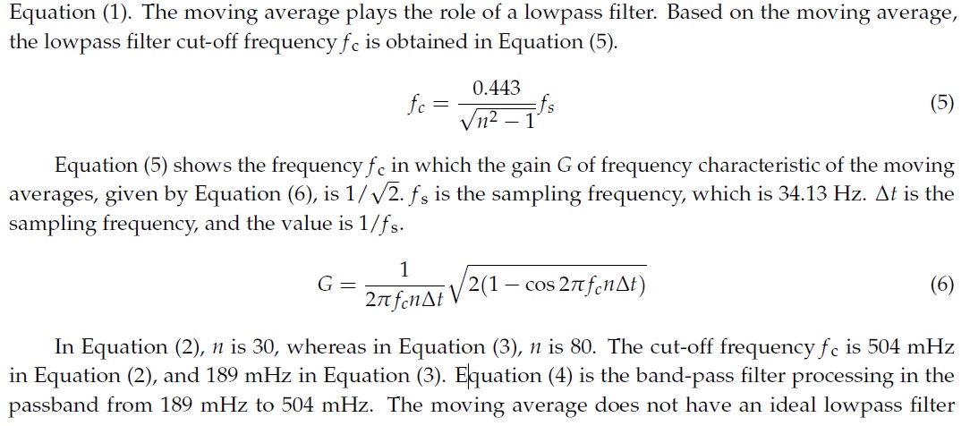
to obtain the window size for their moving average filters they applied the following equation:

I couldn't quite understand where this equation (5) was coming from but as soon as you replace the value $n$ with 30 or 80 you get the values of the passband cut-off freequencies 189 mHz and 504 mHz.

When I asked for specifications on how they did it, they send me to a japanese forum that unfortunately I couldn't translate but there were two links to stackexchange, on cuttoff freequency and filter design.

I tried to adapt all these new staff on my model but couldn't get the passband wanted (0.1 Hz - 0.8 Hz) using the equation (5) from the image above with my parameters (sampling freequency of 50Hz, cut-off freqs etc...).

I don't understand what is the problem and my question is the following:

What are the moving average filter windows that I have to use and in which order to be able to filter a signal with a sampling frequency of 50 Hz in order to isolate the frequencies between the passband 0.1 Hz - 0.8 Hz?

Answer 1

The Japanese link actually implies how to derive Eq.5, and ironically they also refer to an existing dsp.se answer at the bottom.

Derivation of Eq.5 is as follows:

Consider a moving average filter of length $N$, with the impulse response $h[n]$:

$$h[n] = \begin{cases} ~~~1/N~~~,~~~n=0,1,...,N-1 \\ ~~~0~~~,~~~ \text{otherwise} \end{cases} \tag{1}$$

Magnitude of its frequency response $~H(\omega)~$ (DTFT of $h[n]$) can be shown to be:

$$ |H(\omega)| = \frac{1}{N} \left|\frac{ \sin(\frac{\omega}{2}N)}{\sin(\frac{\omega}{2})}\right| \tag{2}$$

Now, after replacing the $\sin()$ functions with their Taylor expansions in powers of $\omega$, it can be shown by polynomial long division that Eq.2 is also given by :

$$|H(\omega)| = 1 + \frac{1}{24}(1-N^2) \omega^2 + H.O.T. \tag{3}$$ where H.O.T. refers to higher order terms in powers of $\omega$. An approximation for small values of $\omega$ is obtained by neglecting H.O.T.:

$$|H(\omega)| \approx 1 + \frac{1}{24}(1-N^2) \omega^2 \tag{4}$$

Using this approximate frequency response magnitude, we can obtain an approximate cutoff frequency $\omega_c$ at which the magnitude $|H(\omega_c)|$ falls to $1/\sqrt{2}$ of its value at $\omega = 0$, which is $H(0) = 1$.

$$ |H(\omega_c)| = \frac{1}{\sqrt{2}} = 1 + \frac{1}{24}(1-N^2) \omega_c^2 \tag{5}$$

Replace the discrete-time frequency $w_c$ by $w_c = 2\pi f_c /f_s$, where $f_c$ is the analog cutoff frequency in Hz, and $f_s$ is the sampling frequency in Hz. Finally solving the resulting algebraic expression for $f_c$ yields the formula that you refer to as Eq.5 in the document :

$$ |H(\omega_c)| = \frac{1}{\sqrt{2}} = 1 + \frac{1}{24}(1-N^2) \left( 2\pi \frac{f_c}{f_s} \right)^2 \tag{6}\\\\$$

$$ f_c = \frac{1}{\pi} \frac{\sqrt{6 - 3\sqrt{2}}}{\sqrt{N^2-1}} ~f_s ~~ =~~ \frac{0.422}{\sqrt{N^2-1}} ~f_s \tag{7} $$

Eq.7 above is the formula that provides an approximate cutoff frequency calculation for the moving average filter of length $N$ (order $N-1$). In your posted link, Eq.5 there's a slight variation at the scale of $0.442$ instead of $0.422$, probably they tried to apply some correction to the actual cutoff vs approximated one.

Note that in the derivation, we've used an approximation of the DTFT magnitude which was valid as long as $\omega$ was small compared to $\pi$. This means that the approximation will be satisfactory if $\omega_c$ is close to $0$, or in other words, $f_c$ is a small compared to $f_s$. And indeed this will be the case for high order moving average filters. And the approximation gets better as $N$ increases.

Using such two moving average filters with approximate cutoff frequencies $f_{c1}$ and $f_{c2}$ to create a bandpass filter will not be very satisfactory unless your out of band signal energy is insignificand after 20 to 30 dB of attenuation.