2
$\begingroup$

what exactly happens when I increase the sampling period ?

Providing some Matlab plots so that I can be more clear.

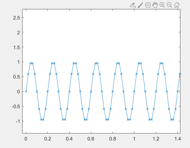
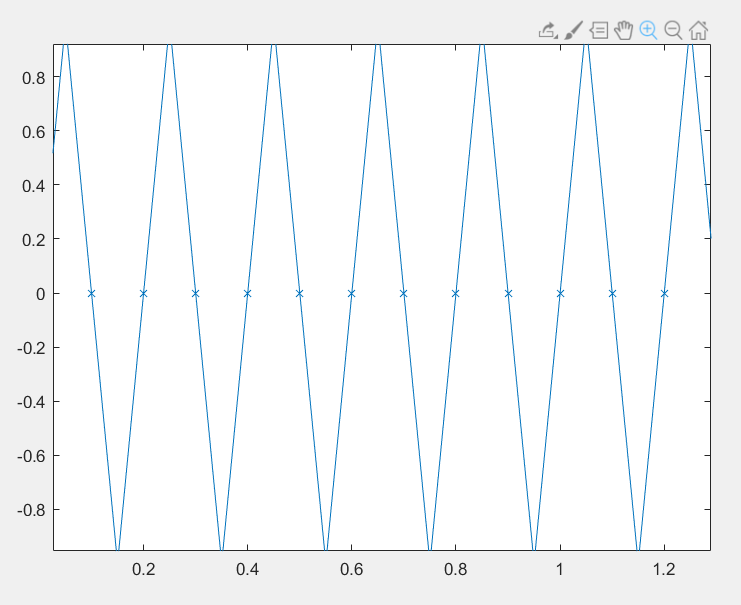
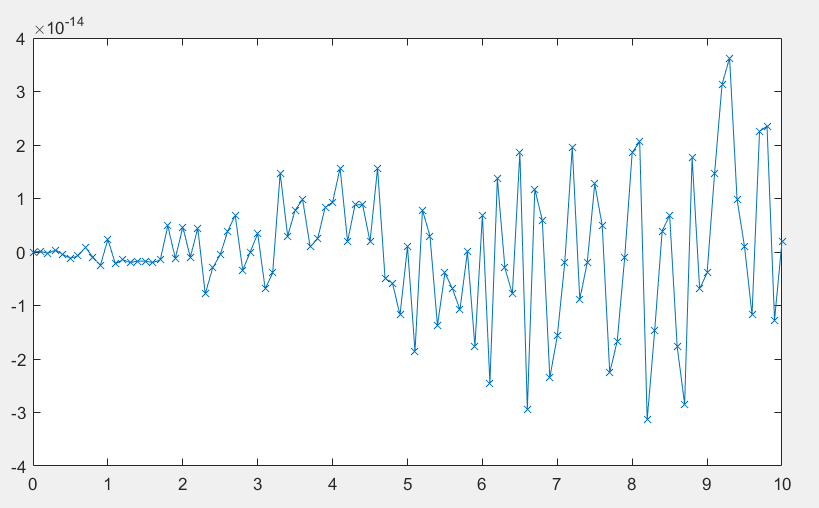
Using the signal $x(t) = \sin(10\pi t)$ and periods $T_s=0.02 ,\; 0.05 ,\; 0.1$

0.02

0.05

0.1

What happens exactly to the signal when the $T_s = 0.1s$ ?

$\endgroup$
1
  • $\begingroup$ Hint: the third chart is vertically scaled to much smaller values. $\endgroup$ Commented May 18, 2020 at 15:44

3 Answers 3

4
$\begingroup$

You sample at times $nT_s$, so the values of the sampled signal are

$$x_d[n]=x(nT_s)=\sin(10\pi nT_s)\big |_{T_s=0.1}=\sin(n\pi)=?$$

Can you take it from here?

$\endgroup$
3
2
$\begingroup$

You are sampling a sine function that should return zero, but because of finite precision argument into that sine function, the error tends to increase towards the right?

$\endgroup$
2
$\begingroup$

Your x-axis is apparently varying between plots. And Matlab plots joining lines between discrete points are misleading. So, here is an other version, with more sampling times:
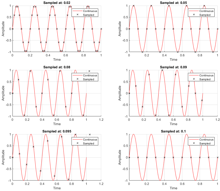
A sine at different sampling times

The Nyquist-etc sampling theorem tells you (somehow) that if you don't have at least two samples per period, you are likely to loose most of the signal's information. Until $0.095$ sampling, although you seem to sometimes loose on dynamics, you still have theoretical hope (if the discrete signal were infinite, etc.) that you can recover the continuous data. Yet, as the sampling time increases, it become more difficult to imagine the red signal from the black crosses. And indeed, as time sampling reaches $1/(2*5)$ (the $5$ as in $\sin(2 \pi 5 t)$), almost all is lost, as you can see from the unscaled graphs, very close to zero for the last one:
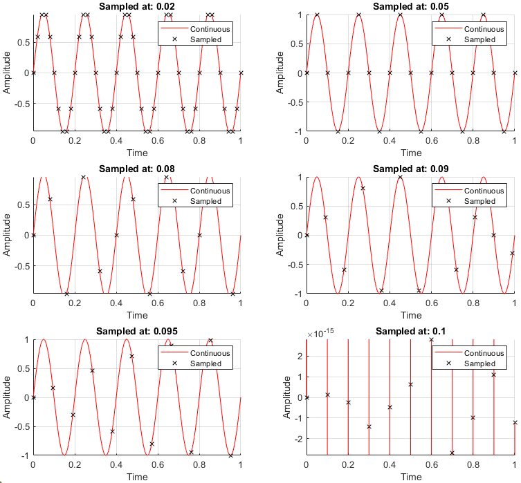
A sine at different sampling times unscaled

$\endgroup$

Your Answer

By clicking “Post Your Answer”, you agree to our terms of service and acknowledge you have read our privacy policy.

Not the answer you're looking for? Browse other questions tagged or ask your own question.