Disagreement between Analytic Convolution and FFT Convolution

Question

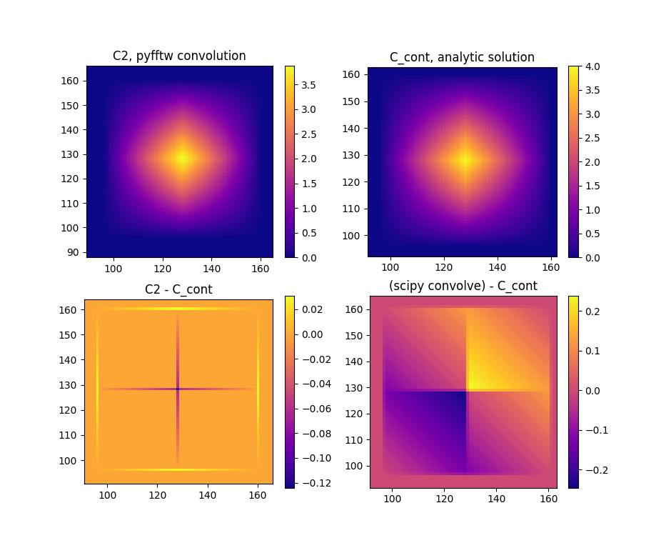
I've been working on a small project, and as a part of this I need a function that can compute the structure function of the input data. In the process of writing this part/testing it I found the results were actually a poor match to what I would expect based on an analytic solution. Upon some further investigation, I've found this mismatch applies even to 2D convolutions and I have been completely stuck trying to debug this.

The test case that I am running is two rectangular functions convolved with one another, my expected result is a 2D triangle function (a pyramid essentially). But the difference between the analytic output and the FFT convolution output is large enough that I am concerned something is wrong. Furthermore, when I compute a direct convolution of the two inputs using scipy.convolve I get yet another output, different from the other two in it's own unique way!

To demonstrate the differences I'm seeing, I've plotted: my FFT Convolution's output, the analytic solution, the difference between them, and the difference between scipy.convolve's output and the analytic solution. My question then boils down to a couple things:

• How large of a difference is expected between the FFT convolution and the analytic solution?
  • I would have expected something small (of order 1e-15 or less) but the peak difference I am seeing is 0.12. It also follows a very particular pattern, the vast majority of the output is close enough (difference of ~1.0e-16).
• Is there a key step or concept that I am missing here?
  • I've been taking the FFT of each input, multiplying them together, and then taking the inverse FFT (with some scaling based on pixel size).

The code that produces the figure can be found in this relatively simple jupyter notebook on my github.

Answer 1

After playing with the notebook for a while, I figured out the following:

1. The result from scipy is shifted by one pixel in each axis (probably due to its definition of the "same" mode). Or, alternatively, both the analytic result and pyfftw results are shifted the opposite way.

   After working around that, the result is exactly (within error) the same as the pyfftw result. I did this as follows (though this drops some data on the edges):

B_padded = np.pad(B, ((0, 1), (0, 1)), 'edge')[1:, 1:]
C1 = scipy.signal.convolve(A, B_padded, 'same', 'direct') * delta**2

2. The analytic solution (which peaks at 4.0) is not quite right for your input data (31x31 pixels at 1.0, edges at 0.5, and corners at 0.25). The peak value (where the image and the window align perfectly) should be:

box_bulk = 1.0**2 * (31 * 31)
box_edges = 0.5**2 * 31 * 4
box_corners = 0.25**2 * 4
peak = (box_bulk + box_edges + box_corners) / 1024 * 4  # ~= 3.876

which is the answer produced by both scipy and pyfftw.

Gist (also includes plotting tweaks).

_{(disclaimer: friend of asker)}