I would take approach based on Blind Deconvolution.
Since we're dealing with ill posed problem some assumptions should be made.
The intuitive approach would be using the information as a prior for the signal. Another idea is to add LPF assumption of the Filter by setting the sum of its coefficients to be 1 and non negative. Yet since we have Discrete Prior on the signal we're getting into combinatoric problem.
Which means brute force solution where the number of combinations is $ {2}^{n} $ where $ d $ is the number of the signal samples.
For $ n \leq 16 $ I'd say it would work for the given input size.
Yet for solution with higher number of samples this method isn't feasible.
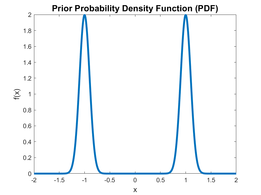
In order to deal with higher dimensions (More samples) I'd use a GMM:

Namely the Prior model is a Gaussian Mixture Model (GMM) with 2 Gaussian's centered at $ \left\{ -1, 1 \right\} $ with very small variance in order to approximate discrete probability function.
So the problem I'm looking to solve is given by:
$$\begin{aligned}
\arg \min_{h, x} \quad & \frac{1}{2} {\left\| h \ast x - y \right\|}_{2}^{2} \\
\text{subject to} \quad & \sum h = 1, \, h \succeq 0
\end{aligned}$$
Step 1 - Solving for the Filter $ h $
Given the signal $ x $ is known, solving for the filter is pretty easy using matrix form of the problem (Which is convex):
$$\begin{aligned}
\arg \min_{h} \quad & \frac{1}{2} {\left\| X h - y \right\|}_{2}^{2} \\
\text{subject to} \quad & \sum h = 1, \, h \succeq 0
\end{aligned}$$
I showed, code included, how to solve such problem in my answer to How to Project onto the Unit Simplex as Intersection of Two Sets (Optimizing a Convex Function)?
Step 2 - Solving for the Signal $ x $
The model is $ y \mid h \sim \mathcal{N} \left( h \ast x, {\sigma}_{n} I \right) $ and the prior $ {x}_{i} \sim 0.5 \mathcal{N} \left( {\mu}_{1} = -1, {\sigma}_{1}^{2} = {0.1}^{2} \right) + 0.5 \mathcal{N} \left( {\mu}_{2} = 1, {\sigma}_{2}^{2} = {0.1}^{2} \right) $.
I'd use the MAP so we have:
$$\begin{aligned}
\arg \max_{x} p \left( x \mid y \right) & = \arg \max_{x} p \left( y \mid x \right) p \left( x \right) \\
& = \arg \max_{x} \log p \left( y \mid x \right) + \log p \left( x \right) \\
& = \arg \min_{x} -\log p \left( y \mid x \right) - \log p \left( x \right) \\
& = \arg \min_{x} \frac{1}{2} {\left\| h \ast x - y \right\|}_{2}^{2} - \lambda \log p \left( x \right) \\
& = \arg \min_{x} \frac{1}{2} {\left\| h \ast x - y \right\|}_{2}^{2} - \lambda \sum \log p \left( {x}_{i} \right)
\end{aligned}$$
Where $ \lambda \propto N {\sigma}_{n}^{2} $ where $ N $ is the number of samples (Dimension of $ y $).
This can be solved by any solver. I'd use MATLAB's fminunc().
Though one could alter (For MAP Estimation) the Expectation Maximization (EM) process for faster and better converging algorithm. Another option would be using Probabilistic Programming with one of the options available today.
Remark: The above is Bayesian Modeling of the problem. One could build optimization problem with some intuition in the form of:
$$ \arg \min_{h, x} \frac{1}{2} {\left\| h \ast x - y \right\|}_{2}^{2} + \lambda \sum_{i = 1}^{m} {\left( {x}_{i}^{2} - 1 \right)}^{2} $$
Which isn't motivated by Bayesian model but still drives the solution to where we want it.
Initialization
One approach to initialization of the estimated $ x $ signal is to use hard threshold. So we set $ {x}_{i} = 1 $ if $ {y}_{i} \geq 0 $ and $ {x}_{i} = -1 $ otherwise.
This approach could also be a greedy method to solve the step for $ x $. Yet it doesn't take under account the delay of the filter.
After iterating enough for a stable solution one could round the result of $ x $ such that $ {x}_{i} \in \left\{ -1, 1 \right\} $.
I haven't tested this approach myself, but I really like its model.
I will publish the results of MATLAB simulation soon.

