If you have a vector that is a superposition of an unknown number of identical Gaussian shaped peaks/impulses of unknown width (but all the same width) and different amplitudes (with Poisson or Gaussian noise), would anyone know of a method to infer this width?
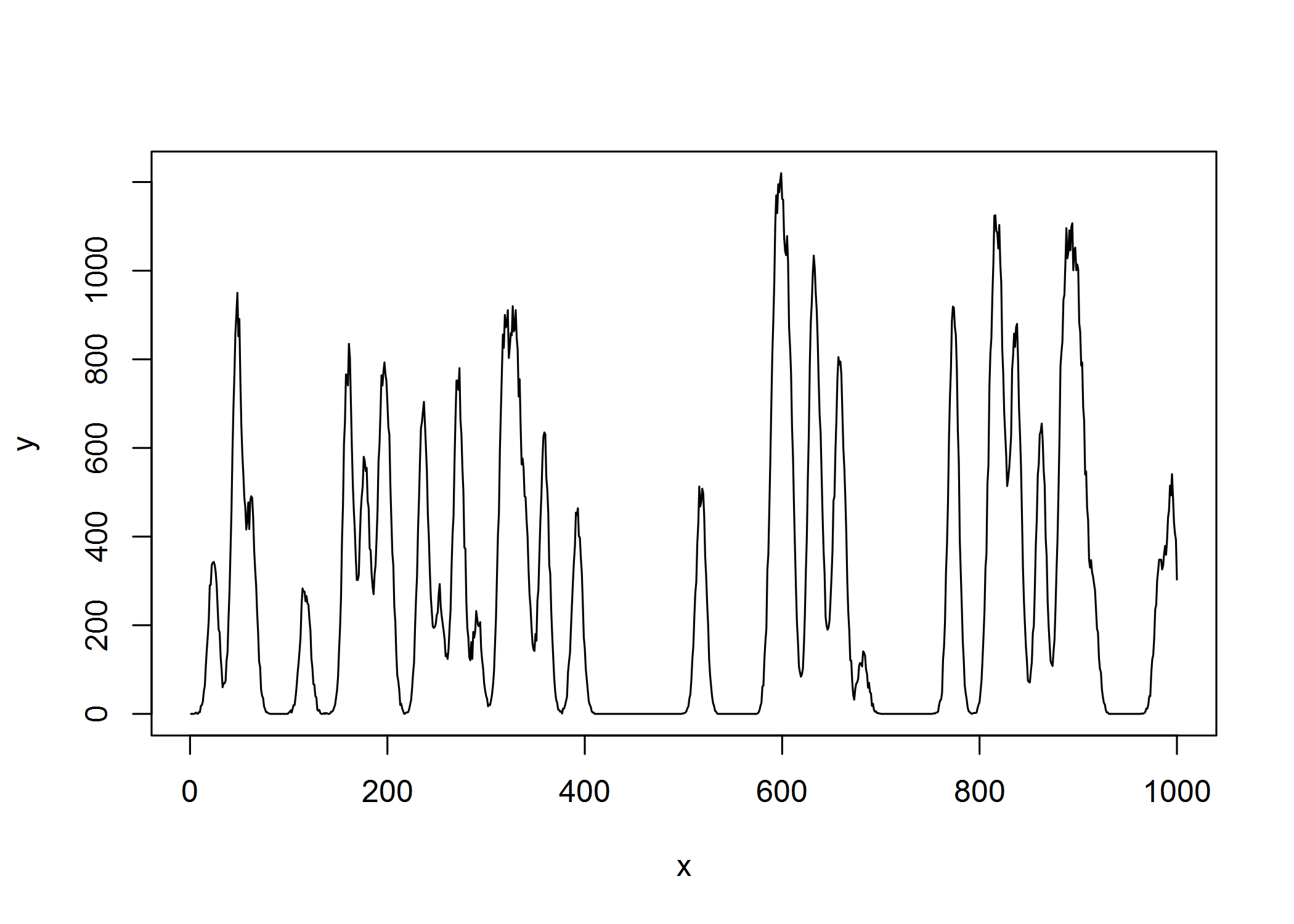
E.g. let's simulate a superposition of Gaussian peaks of width 5 in R:
gauspeak=function(x, u, w, h=1) h*exp(((x-u)^2)/(-2*(w^2)))

sumgauspeaks = function(x, u, w, h) {
  npeaks = length(u)
  n = length(x)
  Y_nonoise = do.call(cbind, lapply(1:npeaks, function (peak) gauspeak(x, u=u[peak], w=w[peak], h=h[peak]) ))
  y_nonoise = rowSums(Y_nonoise)
  set.seed(101)
  Y = apply(Y_nonoise, 2, function(col) rpois(n,col)) # peaks with Poisson noise
  y = rowSums(Y) # measured noisy signal (superposition of identical Gaussians of unknown width & width different heights)
  return(y)
}

x = 1:1000
npeaks = 40 # unknown number of peaks
u = runif(npeaks, min=min(x), max=max(x)) # unknown peak locations
w = rep(5,npeaks) # unknown peak widths (all the same though)
h = runif(npeaks, min=0, max=1000) # unknown peak heights
y = sumgauspeaks(x, u, w, h)
plot(x,y,type="l")
If I measure this (nonnegative) signal in this graph I would then like to be able to estimate that the (constant) peak width w of the superimposed Gaussian peaks in this case was 5 (without knowing a priori their amplitudes/heights or the true number of peaks or their position, but assuming all are identically shaped but differently scaled Gaussians)... Anybody any thoughts how to do this in the most efficient way? Would this be possible e.g. from the DFT or something? Or by estimating a sparse spike train based on a covariate matrix/dictionary with temporally shifted Gaussian peaks of different widths and checking which class of peak width is selected most frequently based on say orthogonal matching pursuit or a LASSO regression? Any thoughts? I just need a rough estimate, it doesn't need to be accurate, but I would like it to be fast...
EDIT: One algorithm that I know of, but which does more than what I want in that it estimates a single best peak shape explaining the signal is that of de Rooi & Eilers (2011) which is implemented in this R code:
# 1. GAUSSIAN PEAK FUNCTION ####
gauspeak=function(x, u, w, h=1) h*exp(((x-u)^2)/(-2*(w^2)))

# 2. FUNCTION TO SIMULATE SUM OF GAUSSIAN PEAKS WITH POISSON NOISE ####
sumgauspeaks = function(x, u, w, h) {
  npeaks = length(u)
  n = length(x)
  Y_nonoise = do.call(cbind, lapply(1:npeaks, function (peak) gauspeak(x, u=u[peak], w=w[peak], h=h[peak]) ))
  y_nonoise = rowSums(Y_nonoise)
  set.seed(101)
  Y = apply(Y_nonoise, 2, function(col) rpois(n,col)) # peaks with Poisson noise
  y = rowSums(Y) # measured noisy signal (superposition of identical Gaussians of unknown width & width different heights)
  return(y)
}

# 3. FUNCTION TO CALCULATE FULL WIDTH AT HALF MAXIMUM OF A FITTED SIGNAL ####
# plus corresponding width of a Gaussian peak function if signal were Gaussian
fwhm = function(x, y, interpol=FALSE) {
  halfheight = max(y)/2
  id.maxy = which.max(y)
  y1 = y[1:id.maxy]
  y2 = y[id.maxy:length(y)]
  x1 = x[1:id.maxy]
  x2 = x[id.maxy:length(y)]
  if (interpol) {
    x.start = approx(x=y1,y=x1, xout=halfheight, method="linear")$y # use spline() if you would like spline interpolation
x.stop = approx(x=y2,y=x2, xout=halfheight, method="linear")$y # use spline() if you would like spline interpolation
  } else {
    x.start = x[which.min(abs(y1-halfheight))]
    x.stop = x[which.min(abs(y2-halfheight))+id.maxy]
  }
  fwhm = x.stop-x.start
  width = fwhm/(2*sqrt(2*log(2)))
  return(list(fwhm=fwhm, width=width))
}

# 4. FUNCTION TO CARRY OUT FAST GAUSSIAN PEAK FIT (USING TER BRAAK / OKSANEN PARAMETERISATION) ####
# i.e. fit  a quadratic model on a log scale using a least square model fit on a log transformed Y scale (if control$fast==TRUE) or using a generalized linear model with Poisson noise fit on a log link scale (if control$fast==FALSE)
# see https://esajournals.onlinelibrary.wiley.com/doi/abs/10.1890/0012-9658(2001)082%5B1191:CIFTOI%5D2.0.CO%3B2
gausfit = function(x, y, control=list(start=NULL, fast=TRUE)) {
  maxy <- max(y)
  if (maxy==0) { return(list(x=x, y=y, fitted=rep(0,length(y)))) }
  if (maxy<=1) { ymax <- 1E5 } else { ymax <- maxy }
  yscaling <- ymax/maxy
  y <- pmax(round(y*yscaling),0)
  ymax_idx <- which.max(y)
  subs_start <- suppressWarnings(max(which(y[1:ymax_idx]==0)))
  if (is.infinite(subs_start)) subs_start <- 1
  subs_stop <- (ymax_idx+suppressWarnings(min(which(y[ymax_idx:length(y)]==0))))
  if (is.infinite(subs_stop)) subs_stop <- length(y)
  subset <- subs_start:subs_stop # y!=0 #  # remove zeros on the side
  x_subs <- x[subset]
  y_subs <- y[subset]
  # we initialize coefficients with weighted least squares model fit on log transformed Y scale
  if (is.null(control$start)) { offs <- 1E-10
                            weights <- y_subs^2/(y_subs+offs)^2
  c <- control$start <- .lm.fit(x=cbind(1,x_subs,x_subs^2)*sqrt(weights),
                            y=log(y_subs+offs)*sqrt(weights))$coefficients
  }

  # now do actual quadratic GLM fit (if fast==FALSE)
  if (control$fast==FALSE) {
c <- suppressWarnings(glm.fit(cbind(1,x_subs,x_subs^2), y_subs,
                              family=poisson(link=log),
                              start=control$start,
                              control=glm.control(epsilon = 1e-8, maxit = 50, trace = FALSE)
))$coefficients
  }

  if (c[[3]]<0) {
    u_fitted <- -c[[2]]/2/c[[3]] # inferred mode
    w_fitted <- sqrt(-(1/2)/c[[3]]) # inferred width
    h_fitted <- exp(c[1] - c[2]^2/4/c[3]) # inferred peak height (* yscaling)
    fitted <- gauspeak(x=x, u=u_fitted, w=w_fitted, h=h_fitted/yscaling)
  } else {
    u_fitted <- mean(x) # inferred mode
    w_fitted <- diff(range(x))/2 # inferred width
    h_fitted <- 0 # inferred peak height (* yscaling)
    fitted <- rep(0,length(x))
  }
  out <- list(x=x, y=y,
              fitted=fitted,
              fitted.pars=c(u=u_fitted, w=w_fitted, h=h_fitted))
  return(out)
}


# 5. DECONVOLUTION FUNCTIONS OF DE ROOI & EILERS 2011 ARTICLE ####
# see https://www.sciencedirect.com/science/article/pii/S0003267011006696

ALS_baseline_fun <- function(y, d = 2, lambda = 10, w = 1, p=0.01){
  m <- length(y)
  E <- diag(m)
  D <- diff(E, diff = d)
  w <- rep(w, m)
  W <- diag(w)
  for (i in 1:20)
  {
    W <- diag(w)
    z <- solve(W + lambda * t(D) %*% D, w * y)
    w <- p * (y > z) + (1 - p) * (y < z)
  }
  return(z)
}


#############################################################
# y = input
# g = given or initial guess of impulse respons
# baseline: 0 = no baseline correction
#               1 = ALS fitting
#               2 = ALS fitting and solving the big system
# gamma = penalty parameter for ALS baseline
# kappa = penalty parameter for deconvolution of the signal
# lambda = penalty for G matrix
# blind: FALSE = impuls respons is taken as given
#          TRUE = impuls response is iteratively improved
#############################################################

deconvol_fun <- function(y, g, baseline=0, gamma, lambda, kappa, k=1, blind=FALSE)
{
  if(baseline!=0)
  {
    # fit baseline
    z <- ALS_baseline_fun(y, d=2, gamma, w=1, p=0.01)
    y <- y - z
  }

  # estimate peaks
  peaks <- L0_peak_fun(y, g, kappa=kappa, blind=blind, lambda=lambda)

  # 'big system' part
  if(baseline==2)
  {
    stop("this function is not yet implemented")
  }
  list(a=peaks$a, g=peaks$g)
}


# actual deconvolution function

L0_peak_fun <- function(y, g, kappa=0.02, blind=FALSE, lambda=0)
{
  nloop = 20
  p = 1
  nc = length(g)
  n = length(y)
  m = n
  w = rep(1, m)
  Gg = matrix(0, nc, nloop)
  for (loop in 1:nloop)
  {
    # Pulsvormmatrix C for fitting
    G = matrix(0, n + nc - 1, n)
    for (k in 1:n) G[(1:nc) + k - 1, k] = g
    G = G[floor(nc / 2) + (1:m), ]

    # Deconvolve
    kappa = kappa
    s0 = 0
    beta = 0.001
    w = rep(1, m)
    for (it  in 1:10)
    {
      W = diag(c(w))
      a = solve(W + t(G) %*% G,  t(G) %*% y)
      w1 = w
      w = kappa / (beta + a^2)
      z = G %*% a
      r = y - z
      s = t(r) %*% r + kappa %*% t(a) %*% a
      ds = s - s0
      if (it == 10) cat(ds, '\n')
      s0 = s
    }

    # Improve C
    if(blind==TRUE)
    {
      G = matrix(0, m + nc - 1, nc)
      for (k in 1:nc) G[(1:n) + k - 1, k] = a
      G = G[(1:m) + floor(nc / 2), ]
      Dg = diff(diag(nc), 1)
      lambda = lambda
      gnew = solve(t(G) %*% G + lambda * t(Dg) %*% Dg, t(G) %*% y)
      g = gnew / max(gnew)
      Gg[, loop] = g
    }

    if (abs(ds) < 1e-6) break
  }
  list(a=a, g=g)
}


# 6. DO TEST ####
x = 1:1000
npeaks = 40
u = runif(npeaks, min=min(x), max=max(x)) # unknown peak locations
w = rep(5,npeaks) # unknown peak widths
h = runif(npeaks, min=0, max=1000) # unknown peak heights
y = sumgauspeaks(x=x, u, w, h)
dev.off()
plot(x,y,type="l")

# estimate peak shape using De Rooi & Eiler's 2011 method
nc=50
g = gauspeak(1:nc, u=25, w=2, h=1) # initial guess of peak shape (peak width guess here too narrow)
system.time(dec <- deconvol_fun(y/max(y), g, baseline=0,
                                lambda=1E-5, kappa=0.01, blind=TRUE)) # takes 149s

dev.off()
par(mfrow=c(3,1))
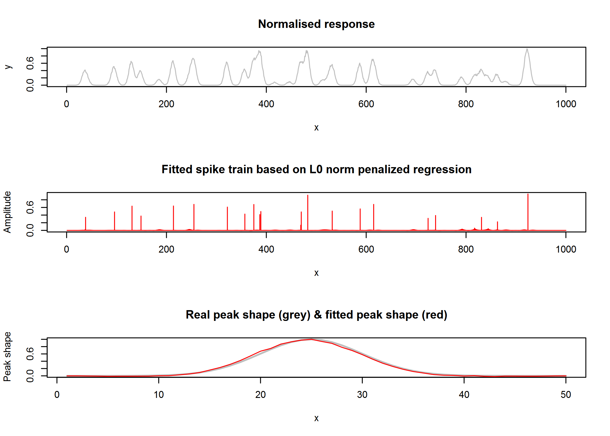
plot(1:length(y), y/max(y),type='l', col="grey", xlab="x", ylab="y", main="Normalised response")
plot(1:length(y), dec$a, type='h', col="red", xlab="x", ylab="Amplitude", main="Fitted spike train based on L0 norm penalized regression")
plot(1:nc, gauspeak(1:50, u=25, w=w[[1]], h=1), type='l', col="grey", lwd=2, xlab="x", ylab="Peak shape", main="Real peak shape (grey) & fitted peak shape (red)")
lines(1:nc, dec$g,type='l', col="red")
fwhm(1:nc, dec$g, interpol=TRUE)$width # estimated width based on full width at half max: 5.10
gausfit(1:nc, y=dec$g, control=list(start=NULL, fast=FALSE))$fitted.pars # estimated width based on Gaussian fit on inferred peak shape: 4.87
For L0 norm penalized regularized / best subset selection I also found this article which I believe is a further development of the Eilers method:
Problems with this algo are that (1) the fitting is not very stable in terms of convergence properties, (2) there are two regularization parameters to tune, (3) that peak shape is not constrained to be Gaussian (could be solved by fitting Gaussian on inferred peak shape after each iteration, but maybe there is a better way??) and (4) the algo is slow (150 s for this small example on my laptop). So ideally I'm looking for something more robust & faster...

