Implementation
Assuming you already have a line drawing routine, you just need to supplement that with some kind of interpolation. The curves are created by drawing enough interpolated short lines to make the result look smooth. A good starting point would be to use an existing interpolation routine, like the ones given by Paul Bourke here.
I'll illustrate this using the cubic routines he supplies, since those are some of the simplest that will still give reasonable results. Here's the first one (translated to python) for reference:
def cubic(mu,y0,y1,y2,y3):
    mu2 = mu*mu
    a0 = y3 - y2 - y0 + y1
    a1 = y0 - y1 - a0
    a2 = y2 - y0
    a3 = y1
    return a0*mu*mu2 + a1*mu2 + a2*mu + a3
Each routine has a parameter mu which represents the fractional part of the index you want to interpolate. Depending on the routine, the other parameters will be some number of samples surrounding the index in question. In the cubic case, you'll need four samples. For example, if your data is y[n], and you want the value at 10.3, mu would be .3, and you'd pass in y[9], y[10], y[11], and y[12].
Then instead of drawing a single line with endpoints, say, $(10,y_{10}) \rightarrow (11,y_{11})$, you'd draw a bunch of shorter ones using the interpolated values (e.g. $(10,y_{10}) \rightarrow (10.1,\text{cubic}(.1,y_9,y_{10},y_{11},y_{12})) \dots $). Obviously those points would need to be scaled to the $x$ and $y$ dimensions of the image to be rendered.
Theory
Now, since the page/routine I referenced doesn't cite any sources, it's worth explaining where those cubic routines come from (and how they work). Both the one I reproduced above, and the very similar Catmull-Rom spline he mentions just below it, are two specific cases of using the following cubic convolution kernel:
$$
\psi(x) =
\begin{cases}
(\alpha + 2)|x|^3 - (\alpha + 3)|x|^2 + 1, & \text{ if } 0 \le |x| \lt 1 \\
\alpha|x|^3 - 5\alpha|x|^2 + 8\alpha|x| - 4\alpha, & \text{ if } 1 \le |x| \lt 2 \\
0, & \text{ if } 2 \le |x|
\end{cases}
$$
The routine listed above corresponds to a value of $\alpha = -1$, and the Catmull-Rom spline corresponds to $\alpha = -1/2$. I won't go into too much detail about how the general form of the kernel is derived, but it involves various constraints like making sure that $\psi(x)$ is one at zero, and zero at all other integers.
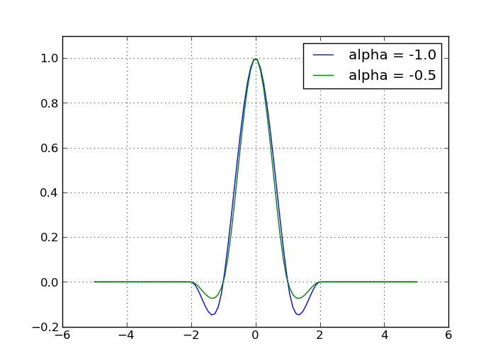
This is what it looks like:

The two choices for the value of $\alpha$ come from attempts to match various aspects of the sinc function, the ideal reconstruction kernel. Setting $\alpha = -1$ makes the derivative of $\psi$ match the derivative of the sinc function at $x = 1$, and making it equal to $-1/2$ provides the best low-frequency approximation instead. By all accounts, a value of $\alpha = -1/2$ has much better properties overall, so it's probably the best value to use in practice. A much more extensive discussion can be found in the following paper, starting on page 328:
Meijering, Erik. “A Chronology of Interpolation: From Ancient
Astronomy to Modern Signal and Image Processing.” Proceedings of the
IEEE. vol. 90, no. 3, pp. 319-42. March 2002.
Insight
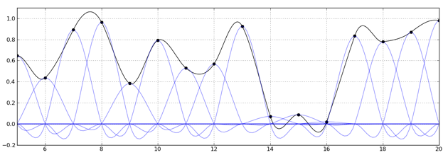
Now, just looking at that kernel in relation to the actual implementation of the interpolation code, it may not be clear how the two are related. Basically, the interpolation process can be thought of as adding together shifted copies of the kernel, which are scaled by the samples of the data, like so:

In fact, if you have an implementation of the kernel, you can use it directly to do the interpolation, as follows:
def kernel(x, a=-1.0):
    x = abs(x)
    if x >= 0.0 and x < 1.0:
        return (a + 2.0)*x**3.0 - (a + 3.0)*x**2.0 + 1
    elif x >= 1.0 and x < 2.0:
        return a*x**3.0 - 5.0*a*x**2.0 + 8.0*a*x - 4.0*a
    else:
        return 0.0

def cubic(mu,y0,y1,y2,y3):
    a = -1.0
    result  = y0 * kernel(mu + 1, a)
    result += y1 * kernel(mu, a)
    result += y2 * kernel(mu - 1, a)
    result += y3 * kernel(mu - 2, a)
    return result
However, it's much less computationally efficient to do it that way. As a bridge from the direct kernel approach to the more streamlined one above, consider that with a little bit of algebraic manipulation, the first implementation can be put in the following form:
def cubic(mu,y0,y1,y2,y3):
    mu2 = mu*mu
    mu3 = mu*mu2
    c0 = -mu3 + 2*mu2 - mu
    c1 =  mu3 - 2*mu2 + 1
    c2 = -mu3 + mu2 + mu
    c3 =  mu3 - mu2
    return c0*y0 + c1*y1 + c2*y2 + c3*y3
In this formulation, the c0...c3 values can be thought of as the coefficients of an FIR filter which is applied to the sample values. Now it's much easier to see how to derive the routine from the kernel. Consider the kernel with $\alpha = -1$, like so:
$$
\psi(x) =
\begin{cases}
|x|^3 - 2|x|^2 + 1, & \text{ if } 0 \le |x| \lt 1 \\
-|x|^3 + 5|x|^2 - 8|x| + 4, & \text{ if } 1 \le |x| \lt 2 \\
0, & \text{ if } 2 \le |x|
\end{cases}
$$
Now evaluate that kernel symbolically at various shifted offsets, keeping in mind that mu ($\mu$) ranges from 0 to 1:
$$
\begin{eqnarray}
\psi(\mu + 1) &=& -(\mu + 1)^3 + 5(\mu + 1)^2 - 8(\mu + 1) + 4 &=& −\mu^3 + 2\mu^2 - \mu & & (c_0) \\
\psi(\mu) &=& \mu^3 - 2\mu^2 + 1 &=& \mu^3 - 2\mu^2 + 1 & & (c_1)\\
\psi(\mu - 1) &=& (1 - \mu)^3 - 2(1 - \mu)^2 + 1 &=& -\mu^3 + \mu^2 + \mu & & (c_2)\\
\psi(\mu - 2) &=& -(2 - \mu)^3 + 5(2 - \mu)^2 - 8(2 - \mu) + 4 &=& \mu^3 - \mu^2 & & (c_3)\\
\end{eqnarray}
$$
Note that $\mu - 1, \mu - 2$ get "flipped" to $1 - \mu, 2 - \mu$ respectively because of the absolute value on $x$ in the kernel definition. Now we have the exact polynomials that are used in the "FIR version" of the interpolation routine. The evaluation of those polynomials can then be made more efficient through standard techniques (e.g. Horner's method). Similar things can be done with other kernels, and there are other ways of constructing efficient implementations as well (cf. Digital Audio Resampling Home Page).


