How about answer your question in an ultimate way? What will happens to if you apply a low pass filter infinite times or practically a large number of times? I believe it is more meaningful for you to understand this one.
I want to first emphasize the fact that apply a filter $F$ to $d$ for $k$ times, is equivalent to apply a filter $F'$ to $d$ for once, if we have
$$F' = \underbrace{F*F*\cdots*F}_{k \,{\rm times}} $$.
The answer to the 'ultimate' version of your question is that: no matter where you start with your lowpass filter, say $F=[f_0,f_1,\cdots,f_n]$, with $\sum_{i=0}^{n} f_i = 1$ and $f_i \geq 0$, you will end up to apply a Gaussian filter $G$ when you apply filter $F$ to some discrete signal $d=[d_0,d_1,\cdots,d_m]$ for $k\rightarrow\infty$ times.
Note: this conclusion does not rely on
1) what is the signal to be processed $d$,
2) which $F$ you use, as along as it is lowpass.
Here is some ipython code, you might play with.
import numpy as np
# generate a random low pass filter
F = np.random.randint(0,1000,(100,1) ).astype('float').ravel();
# ensures sum to 1
F = F / F.sum();
print "sum(F) = ", F.sum();
# create copy to buffer the last version of convolving F for k times
Fk = F.copy();
Fk_list = [];
for k in range( 5 ) :
    Fk = np.convolve( Fk, F, 'full' );
    Fk = Fk / Fk.sum();
    # donot worry about this line, see comments below
    Fk = np.asarray( filter( lambda x : x > 1e-6, Fk ) );
    Fk = Fk / Fk.sum();
    Fk_list.append( Fk );
# plot results
f, axarr = pyplot.subplots( 3, 2 );
# plot data
axarr[0,0].plot( F ),
axarr[0,0].set_title( 'k = 0' );
axarr[0,1].plot( Fk_list[0] ),
axarr[0,1].set_title( 'k = 1' );
axarr[1,0].plot( Fk_list[1] ),
axarr[1,0].set_title( 'k = 2' );
axarr[1,1].plot( Fk_list[2] ),
axarr[1,1].set_title( 'k = 3' );
axarr[2,0].plot( Fk_list[3] ),
axarr[2,0].set_title( 'k = 4' );
axarr[2,1].plot( Fk_list[4] ),
axarr[2,1].set_title( 'k = 5' );
pyplot.show();
- the line that with filter keyword is simply to discard very small components, because I want to keep you see beautiful bell shape Gaussian. Otherwise, the results are still Gassuian, but since we might include many things outside of 4 times of standard deviation, you will see something like a peak instead.
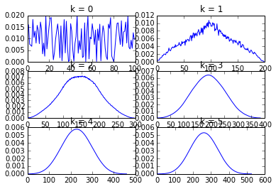
Here are the results of the above ipython code. As you can see, the more times of convolve to $F$ self, the resulting lowpass filter is more similar to a Gaussian.

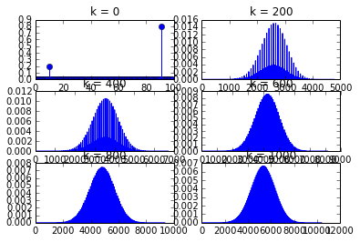
Now let me give you another visual demonstration by using a very different $F$, which only contains two nonzero values. Though this time you cannot see $F$ to be Gaussian like in 5 times of convolution, the long term behaviour namely, $k\rightarrow\infty$ does not change. It will be Gaussian like after a large number of self-convolution.

Finally, you might ask why this thing happens? Because God loves Gaussian. This conclusion is so-called the 'Central Limit Theorem' ( see details in http://en.wikipedia.org/wiki/Central_limit_theorem ). I am not gonna to explain everything for you, because I wish you could learn this on your own. But here is a hint: probability / discrete distribution, arithmetic mean, low-pass filter coefficients, linear operators, and convolution, they are all related. If you have any difficulty to understand something new, try to understand it via something you already knew with close relationships.


