FFT Processing Gain

Question

When transforming a noisy signal via Fast Fourier Transform from time to frequency domain there is a "Processing gain" of the FFT which increases as number of bins increases. I.e. the more bins I have the more the noise floor in the freqeuency domain is reduced.

1. Actually I don't understand completely, from where this gain is coming from. Does this mean that I need just sample the signal with higher sampling rate in order to have more bins, hence a higher FFT processing gain?

2. What is about the inverse FFT? Do I have a "Processing lost"? When starting in frequency domain does this mean, the more frequency samples I have, the more noise will appear in the time domain signal? However, this would be counter-intuitive since this would also lead to big distortion of signals when applying padding (of the frequency-domain data) for time-domain interpolation purposes.

Answer 1

I think the easiest way to wrap around a concept is to have a simple example:

% example of FFT of a very noisy sin wave
f0 = 1000;     % sinusoid frequency
Fs = 10000;    % sampling frequency 
n = 0:1/Fs:1; % one second worth of sample index
N = length(n);
SNR = -20;    % signal to noise ratio is -20dB
Pn  = 0.5*10^(-SNR/10); % signal power is 0.5 for sin wave
NFFT = round([N/8 N/4 N/2 N]); % FFT size to see how it effects the gain


%% signal and generation
sx = sin(2*pi*f0*n);
sn = sqrt(Pn)*randn(1, N);
%% adding noise
xn = sx + sn;
%% signal with and w/o noise in time
figure(1);
plot(n(1:100), xn(1:100)); hold on;
plot(n(1:100), x(1:100), 'r');
legend('noisy', 'clean');
%% FFT of different sizes
figure(2); 
Xf = fft(xn, NFFT(4));
plot(Fs*(0:NFFT(4)-1)/NFFT(4), abs(Xf)/N, '.-'); hold on;
Xf = fft(xn, NFFT(3));
plot(Fs*(0:NFFT(3)-1)/NFFT(3), abs(Xf)/N, 'r.-');
Xf = fft(xn, NFFT(2));
plot(Fs*(0:NFFT(2)-1)/NFFT(2), abs(Xf)/N, 'g.-'); 
Xf = fft(xn, NFFT(1));
plot(Fs*(0:NFFT(1)-1)/NFFT(1), abs(Xf)/N, 'k.-');
legend('FFT size = N', 'FFT size = N/2', 'FFT size = N/4', 'FFT size = N/8');

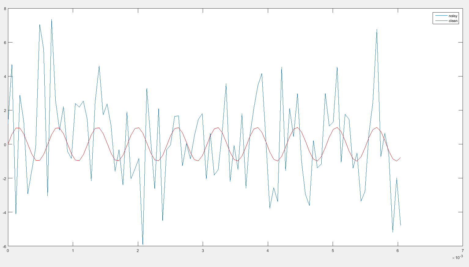
The plot of noisy and clean sin wave in time domain looks like this:

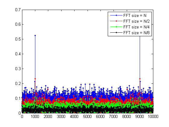
The FFT plots for different sizes in frequency domain is:

i.e., increasing the FFT size means adding more signal samples in the calculation, and therefore easier for FFT to determine the frequency, as the signal information gets added on, while the noise information does not. Here you can see the "relative" noise floor w.r.t signal has decreased.

As for inverse Fourier, I won't say it is a loss, I'd say we went back where we came from.

hth.

Answer 2

The "'Processing gain' of the FFT which increases as number of bins increases" is due solely to an issue of definition. the FFT is a "fast" algorithm to compute the DFT. usually the DFT (and inverse DFT) is defined as:

$$ X[k] \triangleq \sum_{n=0}^{N-1} x[n] e^{-j 2 \pi n k/N} $$

and

$$ x[n] = \frac{1}{N} \sum_{k=0}^{N-1} X[k] e^{+j 2 \pi n k/N} $$

but it could have been defined as

$$ X[k] \triangleq \frac{1}{N} \sum_{n=0}^{N-1} x[n] e^{-j 2 \pi n k/N} $$

and

$$ x[n] = \sum_{k=0}^{N-1} X[k] e^{+j 2 \pi n k/N} $$

and can even be defined as

$$ X[k] \triangleq \frac{1}{\sqrt{N}} \sum_{n=0}^{N-1} x[n] e^{-j 2 \pi n k/N} $$

and

$$ x[n] = \frac{1}{\sqrt{N}} \sum_{k=0}^{N-1} X[k] e^{+j 2 \pi n k/N} $$

in the latter form, there is no "processing gain" of either the DFT nor iDFT.

Answer 3

Let's look at the effect of an FFT on a coherent signal, and then compare it to the effect it has on a random Gaussian noise sequence. First, consider a coherent signal, such as $x[n] = \sigma_{s} \sin[\omega_{0} n]$. The N-point DFT of the signal is $$ X[k] = \sum_{n=0}^{N-1} x[n] e^{-j 2 \pi n k / N}. $$ Suppose $\omega_{0} = 2\pi (10) / N$, so the $X[10]$ is the bin corresponding to our signal. That is $$X[10] = \sum_{n=0}^{N-1} \sigma_{s} \sin(2 \pi 10n/N ) e^{-j 2 \pi 10 n/ N} =\sigma_{s} \sum_{n=0}^{N-1} \sin(2 \pi 10 n/N ) (\cos{2 \pi 10 n/ N} - j \sin{2 \pi 10 n/ N}) , $$ where I used Euler's formula and $\cos(-x) = \cos(x)$ and $\sin(-x) = -\sin(x)$.

Now use $\sin^{2}(x) =1$ and $ 2 \sin x \cos x = \sin 2x$ to get $$ X[10] = \sigma_{s} \sum_{n=0}^{N-1} \frac{1}{2}\sin{ 4 \pi 10 n/ N} - j \sigma_{s} \sum_{n=0}^{N-1} 1 . $$ The real part of $X[10]$ (the first sum) is just the sum of an oscillating series, and so it's value will be small as long as $N$ is of reasonable size. The imaginary part of $X[10]$ is equal to $ - \sigma_{s} N $.

The power corresponding to our signal is then $$|X[10]|^{2} = Re(X[10])^{2} + Im(X[10])^{2} \approx \sigma_{s}^{2} N^{2}.$$

Now let's see what happens to an incoherent sequence of uncorrelated random values with variance $\sigma_{n}^{2}$, $y[n]\sim\mathcal{N}(0, \sigma_{n}^{2})$. The N-point FFT is now $$ Y[k] = \sum_{n=0}^{N-1} y[n] e^{-j 2 \pi kn / N} . $$ Of course, $Y[k]$ is also a random variable. Let's look at the expected value of its power. $$ E(|Y[k]|^{2}) = E\left[\left(\sum_{n=0}^{N-1} y[n] e^{-j 2 \pi nk / N}\right)\left(\sum_{n=0}^{N-1} y[n]^{*} e^{j 2 \pi nk / N}\right)\right] = \left(\sum_{n=0}^{N-1} E(|y[n]|^{2}) \right) + \left( \sum \sum _{i \neq j} E(y[i] y[j]^{*}) e^{j 2\pi (j-i)/N} \right) $$ (I factored the product into two sums, and used linearity of expectation).

Now, $E(|y[n]|^{2}) = \sigma_{n}^{2}$, and since $y[n]$ is assumed uncorrelated from sample to sample, $E(y[i]y[j]$, with $i\neq j$, is simply 0.

Therefore, $$ E(|Y[k]|^{2}) = \sigma_{n}^{2} N $$.

SNR is the ratio of signal power to noise power. Since the noise is described statistically, the SNR is also a random variable. Its expected value increases as the FFT length increases. This is because the FFT coherently sums the signal, while it randomly sums the noise. Specifically, $$ SNR = \frac{|X[10]|^{2}}{|Y[10]|^{2}} = \frac{\sigma_{s}^{2}}{\sigma_{n}^{2}} N .$$ We can see that the SNR increases as N. If we define the input SNR to be, in decibels, $SNR_{input} = 10 \log_{10}\frac{\sigma_{s}^{2}}{\sigma_{n}^{2}}$ we get that, in dB, $$ SNR_{db} = SNR_{input} + 10 \log_{10} N .$$ This is the $10 \log_{10} N$ gain that an FFT has on a coherent signal over a random noise signal.

Answer 4

The FFT processing gain comes from the fact that the DFT (of which FFT is simply a fast implementation) is a non-normalized linear transformation. This is a mouthful, so let's look at what this means.

I'm going to assume that you know what a linear transformation is. Namely, given vectors $\mathbf{x}$ and $\mathbf{y}$ and a matrix $A$ we have

$$\mathbf{y} = A \mathbf{x}.$$

DFT is just such a transformation. In fact, you can use MATLAB dftmtx command to generate this matrix for you based on the length of vector $\mathbf{x}$. This this case,

$$\mathbf{y} = \text{DFT}(\mathbf{x}).$$

This matrix $A$ has some properties. First of all, it's a square matrix, which means that it's probably invertible (and indeed it is!). It also tells us that we're essentially taking components of x and performing a change of basis given by the columns of $A$ to get its DFT. So far so good.

Now, let's get to some more important properties. Matrix $A$ is orthogonal. This means that every column of $A$ is perpendicular to every other column, or more mathematically, $A^TA$ is a diagonal matrix (you may have to think a little about why this is true). This is a very nice property, since simply transposing the matrix gives us something very close to its inverse.

To make this Transpose $\leftrightarrow$ Inverse relationship strict, we want the matrix $A$ to also be normal. This is a matrix whose every column vector has length 1. In other words, if $a$ is a column of $A$, then $\sqrt{a^Ta} = 1.$ If a matrix is both orthogonal and normal, we call it orthonormal, and in this case $A^TA = I$, so $A^T$ is in fact the inverse of $A$. Neat!

The usual DFT matrix (or the usual DFT transform) is orthogonal, but not orthonormal. In fact, if $D$ is the DFT matrix, then $D^TD = N$ where $N$ is the number of columns (or rows, it's square!) in $D$. To make it orthonormal, we should use $\frac{D}{\sqrt{N}}$ instead. If you look at it long enough, you realize that is we scale both forward and inverse transforms by $\frac{1}{\sqrt{N}}$, we're doing extra work in performing the calculations, so we usually just scale by $\frac{1}{N}$ at the inverse.

There are better theoretical reasons for doing it on one side rather than of both. See my answer here for more information.

Answer 5

The processing gain of the FFT refers to increased SNR for a sinusoid. You can think of the DFT or the FFT as a bank of matched filters. The matched filter maximizes the SNR at the output. Another way to look at the processing gain, if you have sinusoid in noise in the time domain at a given SNR and then take the FFT and look at the Sinsoid power vs the noise power in the FFT bin (assuming the frequency corresponds exactly with a FFT bin) then you will see a higher SNR or processing gain. You can think of the FFT as bandwidth filters and the noise in each frequency bin is spread out in comparison to the time-domain signal where the noise is through out the signal.

The processing gain comes about because it coherently adds the components of the sinusoid together. So you will also see this called coherent gain. This coherent addition is also why when you have a longer signal you get more processing gain i.e. more samples add together coherently. By coherent I mean that it assumes you have knowledge of the phase of the signal - in this case the frequency. Alternatively you can think of a longer matched filter as having a narrower bandwidth, so less noise gets through the filter. Thus giving you better SNR or processing gain.

Note that if the sinusoid does not exactly align with a frequency of an FFT bin, then there will still be a peak at near by FFT bins, but then a few of the neighbouring FFT bins will also contain significant magnitudes. There will be a peak at the nearest FFT bin but it will be less than the processing gain. This effect is often callled spectral leakage. You can use windows to reduce the spectral leakage, but you decrease the processing gain as well. The worst case loss is when your signal sits exactly between two FFT bin frequencies.

I would suggest you read the Harris paper on windows. It explains a lot of the details I am talking about.

So if you have a sinusoid in white noise you will get the processing gain by taking the DFT/FFT. By taking the IFFT/IDFT you will suffer a processing loss because you are spreading your signal back into the noise.

Answer 6

I have a circuit/ee background and I think the Matlab code from "learner" is very good but not very correct and I would like to correct it based on my own standing. (low reputation hence cannot comment) The FFT results should divided by its own NFFT length instead of divided by N, that's not a correct scaling factor.

In the example, the actual analog signal noise is constant. When there are more FFT bins (higher N), the total noise is distributed into more bins and hence each bin get less noise. The overall noise floor level looks lower but has the same total noise. That's why we should expect to see FFT size = N gets lowest noise floor while FFT size =N/8 has highest noise floor (while the total noise is actually the same for all 4 cases in the analog signal domain)

The FFT process gain is outside of the equation SNR = 6.02N + 1.76dB. This SNR equation (6.02N+.76) only considers quantization noise. The actual signal noise floor before the ADC quantization can be lower than the quantization noise. I think a very good note about this is here (Taking the Mystery out of the Infamous Formula, "SNR = 6.02N + 1.76dB," and Why You Should Care) I still have a few things that I don't understand but thanks to the Matlab code example here.

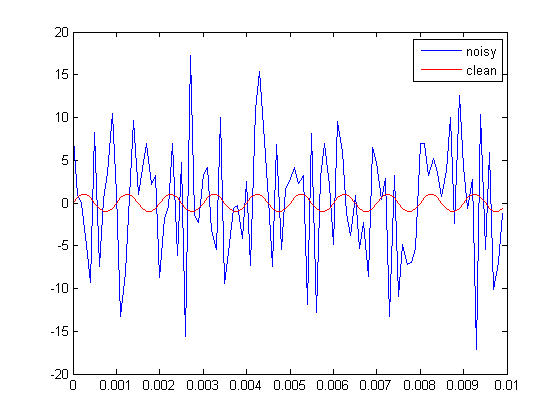
For question 2, I think since FFT and iFFT are linear transform. They should be the same. And with my above explanation, since the noise is actually constant and doesn't change. It doesn't matter transfer between FFT or iFFT.

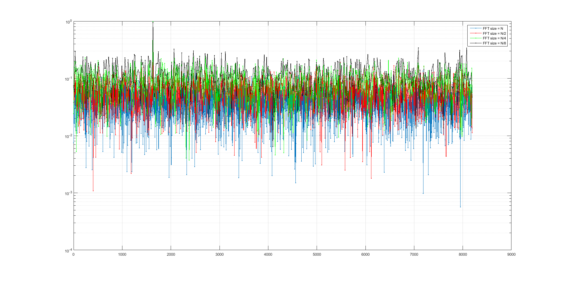
as you can see in this plot, the blue curve with FFT size = N shows lowest noise average level outside of the signal frequency bin. But because it has the largest number of bins. After you summed up all the bins from the blue, you actually get the same noise as all other cases. The FFT size = N/8 has the least number of frequency bins and hence each bin needs to have higher noise to make the total noise equal to other FFT cases.

clear;
close all;
rng default
 
%f1=1e3;
fs=16.384e3;
N=8192;
M=816;
f1=M/N*fs
 
t=0:1/fs:(N-1)/fs;
%t=0:1/fs:1;  %1 second of sampling time
 
NFFT = round([N/8 N/4 N/2 N]); %FFT size
 
amp1=1;
amp_rms1=amp1/sqrt(2);
SNR_dB=-10;
Vnoise=amp_rms1/(10^(SNR_dB/20))
 
sx= amp_rms1*sqrt(2)*sin(2*pi*f1*t);
%sn = Vnoise*randn(1,N);
sn = Vnoise*randn(size(t));
 
xn = sx + sn;
 
figure(1);
plot(t(1:100),xn(1:100));hold on;
plot(t(1:100),sx(1:100),'r')
legend('noisy','clean');
 
%FFT of different size
figure(2)
Xf = fft(xn, NFFT(4));
NFFT_4_FFTresult_length=length(Xf)
P2=abs(Xf)/NFFT(4);
P1=P2(1:NFFT(4)/2+1);
P1(2:end-1)=2*P1(2:end-1);
plot(fs*(0:(NFFT(4)/2))/NFFT(4), P1, '.-');hold on;
 
 
%noise summary
ymax=0;
for i=1:length(P1)
    if P1(i)>ymax
        ymax = P1(i);
    end
end
noiseSum=0;
for i=1:length(P1)
    if P1(i) >= ymax
        % method 1, remove the signal bin
        % below line remove the signal and also the noise from the freq bin        
        %%P1(i) = 0;
        
        % method 2, borrow noise from neighbour bin, not accurate
        %keep the noise on this block
%         if i == 1
%             P1(i)=P1(i+1);
%         else 
%             P1(i)=P1(i-1);
%         end
        % method 3, subtract known signal amplitude from the signal bin
        P1(i) = P1(i)-amp1;
        i
        ymax
    end
    noiseSum=noiseSum+(P1(i)/sqrt(2))^2;
end
%noiseSum
sqrtNoiseSum=sqrt(noiseSum)
    
Xf = fft(xn, NFFT(3));
NFFT_3_FFTresult_length=length(Xf)
P2=abs(Xf)/NFFT(3);
P1=P2(1:NFFT(3)/2+1);
P1(2:end-1)=2*P1(2:end-1);
plot(fs*(0:(NFFT(3)/2))/NFFT(3), P1, 'r.-');
 
Xf = fft(xn, NFFT(2));
NFFT_2_FFTresult_length=length(Xf)
P2=abs(Xf)/NFFT(2);
P1=P2(1:NFFT(2)/2+1);
P1(2:end-1)=2*P1(2:end-1);
plot(fs*(0:(NFFT(2)/2))/NFFT(2), P1, 'g.-'); 
 
Xf = fft(xn, NFFT(1));
NFFT_1_FFTresult_length=length(Xf)
P2=abs(Xf)/NFFT(1);
P1=P2(1:NFFT(1)/2+1);
P1(2:end-1)=2*P1(2:end-1);
plot(fs*(0:(NFFT(1)/2))/NFFT(1), P1, 'k.-');
%noise summary
ymax=0;
for i=1:length(P1)
    if P1(i)>ymax
        ymax = P1(i);
    end
end
noiseSum=0;
for i=1:length(P1)
    if P1(i) >= ymax
        % method 1, remove the signal bin
        % below line remove the signal and also the noise from the freq bin        
        %%P1(i) = 0;
        
        % method 2, borrow noise from neighbour bin, not accurate
        %keep the noise on this block
%         if i == 1
%             P1(i)=P1(i+1);
%         else 
%             P1(i)=P1(i-1);
%         end
        % method 3, subtract known signal amplitude from the signal bin
        P1(i) = P1(i)-amp1;
        i
        ymax
    end
    noiseSum=noiseSum+(P1(i)/sqrt(2))^2;
end
%noiseSum
sqrtNoiseSum=sqrt(noiseSum)
 
legend('FFT size = N', 'FFT size = N/2', 'FFT size = N/4', 'FFT size = N/8');
%yscale log;
set(gca, 'YScale', 'log')
grid on;

Different FFT length separate the sampling frequency fs into smaller frequency bin (or bandpass filter). Each bin has a bandwidth of fs/N For $N/8=1024$, each bin is equal to $16.384e3/1024=16 $ Hz For N=8192, each bin in FFT is equal to $16.384e3/8192=2$ Hz It’s expected that the noise will have spectrum leakage after FFT, but if the signal (not noise) can be contained within the bandwidth of a frequency bin. The purpose of coherent sampling is achieved.

choose $f_1=M/N×f_s=816/8192×16.384e3 = 1632 Hz$

1st frequency bin is at 0 Hz, it will sample signal from 0 to $1*16384/8192$ (including 0 but not including $16384/8192=2$ Hz) Frequency f1 is located at the $(816+1)$th bin, the frequency is same as f1=1632 Hz, it samples signal from $816*16.384e3/8192=1632$ Hz to $817*16384/8192=1634$ Hz.

Because frequency f1 is located at the sampling frequency of the FFT bin, hence there is no spectral leakage, the magnitude of the signal is kept integral.

The FFT based on the matlab code is shown above.

As can be found in the plot, blue curve with FFT size=N shows lower noise floor while FFT size=N/8 shows higher noise floor. While at the same time, the total noise across the whole bandwidth of $fs/2=8192$ Hz is kept constant. The noise rms or standard deviation is 2.236V as calculated above.

So why FFT size =N/8 shows higher noise floor. It’s because the total number of bins existed in this FFT is only N/8=1024. The total noise is divided by this 1024 bandpass filter and distributed into every one of them. As you can see that each frequency bin (bandpass filter) didn’t get the same amount of noise, hence the noise floor is up and down with different value. The calculation in the matlab code with variable name sqrtNoiseSum re-calculates the noise. The value is closed to 2.236V but cannot exactly equal to 2.236V because one of the frequency bins has signal and noise summed up together.

Even if we can remove the signal amplitude from the frequency bin and leave the noise there (method 3 is doing that), the calculated root sum squared noise is still slightly off from 2.236V. I believe that’s due to the spectral leakage. Maybe windowing method can solve this problem but the value is very close to 2.236V already.

For the FFT size = N and FFT size = N/8 cases, the re-calculated noise is equal to 2.2397V and 2.3035V.

The calculated results are not the same each time due to random noise distribution. However, with “rng default” in the Matlab code, the results can be repeated.

Answer 7

The "gain" is in terms of desired (and easy to see) knowledge. If you transform to the frequency domain, you gain more explicit/visible (as can see it in a graphic plot) knowledge of particular frequency bands, but lose visible (can no longer see it in the FFT plot) knowledge of exact timing information. If you transform back to the time domain, then you gain more explicit knowledge of timing (impulse time and transient changes, etc.), but lose visible knowledge (if you throw away the previous FFT plot) of what frequency bands that that time-domain waveform stimulates.

There is no actual gain in the inherent information present in either the time or frequency vector, more likely some tiny loses due to numerical precision within the FFT.

Increase the sampling rate of an already band-limited signal (already below Nyquist at the lower sample rate) adds no new information (except possibly moving the sample data farther from anti-alias filter distortions, and spreading out quantization noise). There's nothing new to which to add more "gain".

But increasing the total sample vector time (not with zero-padding, but with more actual relevant data) can add fresh new information, which may allow processing "gain" to lower the noise floor, especially given a stationary signal.