When deriving the power spectral density of stochastic processes, why does taking an expectation allow the $T\rightarrow\infty$ limit to be taken?

Question

I am following the arguments presented in the paper AN-255 Power Spectra Estimation, from Texas Instruments, to learn how to derive the power spectral density for a stationary stochastic process, and do not understand one of their steps. I am looking at Page 4 only of the the document for the purposes of this question.

The derivation is done by considering only a single realisation (sample function), denoted by $x(t)$, of the stochastic process. Then they do the usual thing of only considering a truncated version of this signal $x_T(t)$, which allows the Fourier transform of it to exist, denoted by $X_T(f)$ (because one of the requirements for FT to exist is absolute integrability, which isn't satisfied for random signals).

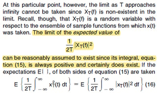
I am confused with how they justify taking the limit $T\rightarrow\infty$ in the right hand column of page 4, shown here:

$\hskip2in$

$\hskip2in$

I understand that you cannot take the limit $T\rightarrow\infty$ directly on the truncated sample function's Fourier transform $X_T(f)$, because it is not defined in that limit (indeed, that was the reason for doing the truncation in the first place).

I also understand that $X_T(f)$ results from a single realisation only of the stochastic process, and if you were to repeat the experiment again you would obtain a different $X_T(f)$. As such, this function is actually a random variable itself (at each frequency $f$), and therefore it makes sense to do an ensemble average over many realisations, and consequently motivates taking an expectation.

What I don't understand is why the expectation solves the problem, and allows you to take the limit $T\rightarrow\infty$ after you have taken the expectation:

$\hskip2in$

What is it about the expectation of $X_T(f)$ that means the limit $T\rightarrow\infty$ can then be taken? I'm having a hard time seeing it... Could someone spell this out plainly for me?

Answer 1

It is not the expectation operator that makes sure that the limit exists. The expectation just results in an ensemble average, which we need to obtain a deterministic function $S(f)$ for the power spectrum.

Assume we're given a deterministic power signal $x(t)$, i.e., a signal with finite non-zero power, and, consequently, infinite energy. Its Fourier transform generally doesn't exist. We can define a truncated Fourier transform

$$X_T(\omega)=\int_{-T}^Tx(t)e^{-j\omega t}dt\tag{1}$$

By assumption, $\lim_{T\to\infty}X_T(\omega)$ doesn't exist. However, the limit

$$\lim_{T\to\infty}\frac{\left|X_T(\omega)\right|^2}{2T}\tag{2}$$

exists because of the finite power assumption, and this is also the way the power spectrum is defined for such deterministic power signals.

If $x(t)$ is modeled as a random signal, we only need to modify $(2)$ by taking the expectation of the numerator to obtain the power spectrum of $x(t)$.

Answer 2

For stationary stochastic signal, taking limit after expectation works as explained below.

You have a windowed random process $x_T(t)$ from which you want to derive the PSD $S_{xx}(f)$ by letting $T \rightarrow \infty$. There are two approaches to this.

(1) You take the $lim_{T \rightarrow \infty} $ on $x_T(t)$ , then compute $|X_T(f)|^2$ and then take Expectation of the it $E(|X_T(f)|^2)$. This fails because $X_T(f)$ does not even exist when $lim_{T \rightarrow \infty}$.

OR

(2) You compute $\frac{1}{2T}|X_T(f)|^2$ from $x_T(t)$ , take expectation over it, i.e., $\frac{1}{2T}E(|X_T(f)|^2)$, then let $lim_{T \rightarrow \infty} \frac{1}{2T}E(|X_T(f)|^2)$.

The second method of taking limit after expectation works because of following reason.

The quantity which you can compute, $ E(|X_T(f)|^2)$, corresponds to $R_{xx}(\tau)W(\tau)$ , which is the expectation of convolution of ACF of $x_T(t)$ and triangular function $w_T(\tau)$. (Remember we did rectangular windowing, so when you compute $|X_T(f)|^2$ you are doing convolution in time domain between $x(t)w_T(t)$ and $x(-t)w_T(-t)$).

When you let $lim_{T \rightarrow \infty}$ the triangular window $W$ becomes square window which results in ACF being $R_{xx}(\tau)$ itself. On the other side of equation, you have $lim_{T \rightarrow \infty}\frac{1}{2T}E(|X_T(f)|^2)$. So, $$ R_{xx}(\tau) \leftrightarrow lim_{T \rightarrow \infty}\frac{1}{2T}E(|X_T(f)|^2) $$

Appendix: $$ |X(f)|^2 \leftrightarrow [x_T(t)w_T(t)]*[x_T(-t)w_T(-t)]\\ E(|X(f)|)^2 \leftrightarrow R_{xx}(\tau)W(\tau)\\ $$ Reference : https://ocw.mit.edu/courses/electrical-engineering-and-computer-science/6-011-introduction-to-communication-control-and-signal-processing-spring-2010/readings/MIT6_011S10_chap10.pdf

For deterministic signals, again approach (1) would fail because $x$ being a finite power signal has infinite energy. Here no assumption is made about $x$ so it is assumed to exist $-\infty \lt t \lt +\infty$. So $lim_{T \rightarrow \infty}$ does not exist.