Wrong matched filter sidelobe level for linear chirp despite (invalid ?) energy normalization

Question

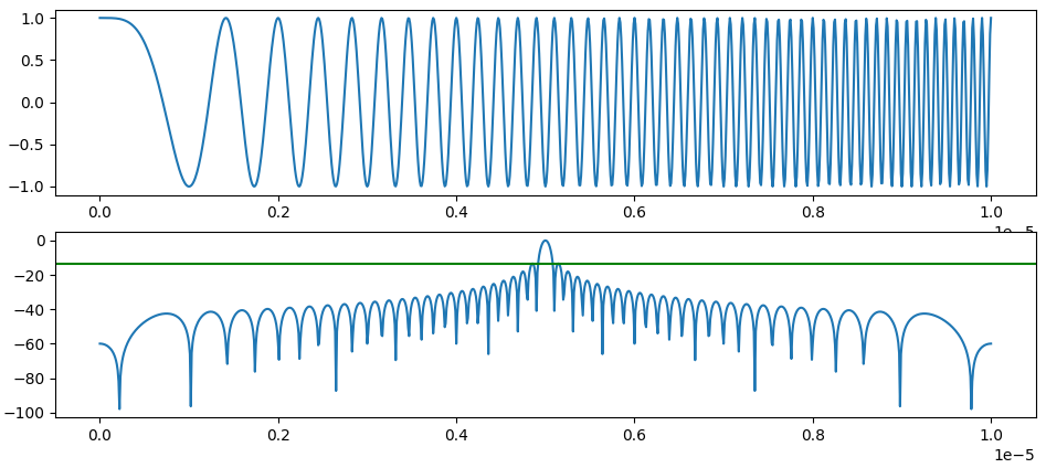
I'm trying to reproduce the -13.2 dB sidelobe level typically observed for a linear chirp pulse (cf. for instance this MATLAB documentation page: the range sidelobes of a linear FM are 13.2 dB below the main lobe.) and always end up with a first sidelobe several dB below despite trying different normalization quantities and both 10*log(abs(corr)) and 20*log(abs(corr)) as dB definition (thought a correlation was already squared so didn't need the 10*log -> 20*log coefficient). I'm additionally confused since the normalization proposed below successfully puts the main lobe peak to 0 dB as expected. Here is the Python code leading to the problematic matched filter profile shown below (green line is -13.5 dB line, substantially above all sidelobes):

import scipy.signal as signal
import numpy as np
import matplotlib.pyplot as plt

fs = 100e6 # sampling freq
BW = 10e6 # LFM chirp bandwidth
T = 10e-6 # pulse duration
t = np.arange(0,T,1/fs)

pulse = np.exp(2j*np.pi*(BW/(2*T))*(t**2))

plt.subplot(2,1,1)
plt.plot(t,np.real(pulse))

pulse_energy = np.sum(np.abs(pulse)**2)

normalized_MF = signal.correlate(pulse,pulse,"same") / pulse_energy

normalized_MF_dB = 20*np.log(normalized_MF)
plt.subplot(2,1,2)
plt.plot(t,normalized_MF_dB)
plt.axhline(np.max(normalized_MF_dB)-13.5,label="Peak - 13.5 dB",color="green")
plt.show()

My understanding is my code is using the following normalization for all delays \tau considered (and my mistake may come from an inconsistent use of the complex-version of the energy computation - which differs from the energy "one-sided" version - w.r.t to the use of |.| to plot magnitudes ?):

Answer 1

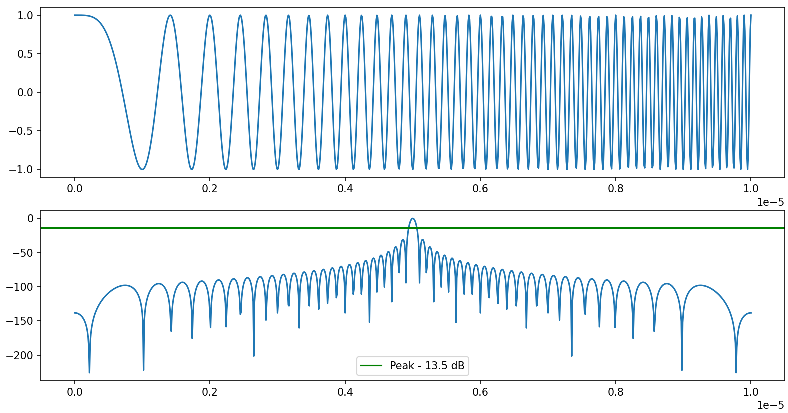
You used the wrong logarithm function. The one in your code is the natural logarithm, not base-10 as intended. The following code produces what is expected:

import scipy.signal as signal
import numpy as np
import matplotlib.pyplot as plt

fs = 100e6 # sampling freq
BW = 10e6 # LFM chirp bandwidth
T = 10e-6 # pulse duration
t = np.arange(0,T,1/fs)

pulse = np.exp(2j*np.pi*(BW/(2*T))*(t**2))

plt.subplot(2,1,1)
plt.plot(t,np.real(pulse))

pulse_energy = np.sum(np.abs(pulse)**2)

normalized_MF = signal.correlate(pulse,pulse,'same') / pulse_energy

normalized_MF_dB = 20*np.log10(normalized_MF)
plt.subplot(2,1,2)
plt.plot(t,normalized_MF_dB)
plt.axhline(np.max(normalized_MF_dB)-13.5,label="Peak - 13.5 dB",color="green")
plt.show()