Python - Discrete deconvolution using Toeplitz matrix

Question

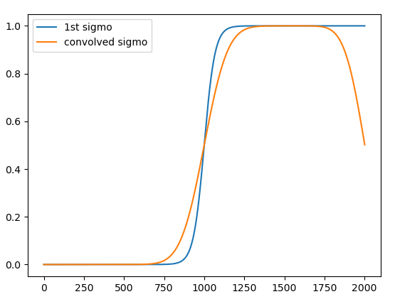
Lets say I have 2 vectors (1D signals that are sigmoids): $s$ and $m$, both related through the relation: $m = s * r$, my goal here is to recover the vector $r$ (should be a gaussian $\rightarrow$ gives the $m$ sigmoid a smoother/steeper slope depending on $\sigma$).

I tried to use Fourier transforms but it did not work very well (see here: https://dsp.stackexchange.com/questions/88801/convolution-and-fourier-transform-for-1d-signals), then tried to use deconvolve from scipy but once again I do not get the right gaussian.

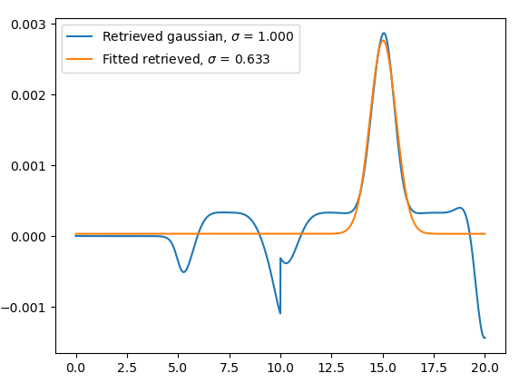
Then someone told me on my last post to look into Toeplitz matrices knowing the following relationship (discrete convolution): $$ m[n] = \sum_{i=0}^{n-1} s[n-k] r[k]$$ we then have n equations with $k$ parameters $\rightarrow$ matrix problem to solve. You'll find below my code using this post: Matlab - Toeplitz matrices. But now I have a problem with my python code as the output does not give a proper gaussian, and if I i fit the peak that looks like one I always get a 2/3 ratio of difference for the standard deviation between the 'real' gaussian used for the convolution and the one I get through this process (see the plots I give both $\sigma$), how could I explain this ?

import numpy as np
import scipy.signal
import matplotlib.pyplot as plt
from scipy.optimize import curve_fit

def sigmoid(x, A, x0, k):
    return A / (1 + np.exp(k * (x - x0)))

def gaussian(x, mu, sigma):
    return np.exp(-((x - mu) ** 2) / (2 * sigma ** 2))

x = np.arange(0., 20.01, 0.01)

# Create a Gaussian signal
mu_gaussian = 10.0
sigma_gaussian = 1.0
y = gaussian(x, mu_gaussian, sigma_gaussian)

# Create a sigmoid-like filter
A_sigmoid = 1.0
x0_sigmoid = 10.0
k_sigmoid = -3.0
sigmo = sigmoid(x, A_sigmoid, x0_sigmoid, k_sigmoid)

sigmo2 = sigmoid(x, A_sigmoid, x0_sigmoid, -0.5)

plt.plot(sigmo, label = '1st sigmo')
plt.plot(sigmo2, label = 'convolved sigmo')
plt.legend()
plt.show()
# yc = scipy.signal.convolve(y, c, mode='full') / c.sum()
# ydc, remainder = scipy.signal.deconvolve(yc, c)
M = len(sigmo2)

# Create the first row of the Toeplitz matrix using the sigmoid values
first_row = np.concatenate((sigmo, np.zeros(M - 1)))
# Create the first column of the Toeplitz matrix with zeros and the first element of `sigmo`
first_col = np.concatenate(([sigmo[0]], np.zeros(M - 1)))

# Generate the Toeplitz matrix
A = scipy.linalg.toeplitz(first_col, first_row)

# # Calculate the product of transpose(A) and A
# product = np.dot(A.transpose(), A)
# # Calculate the inverse of the matrix product
# inverse_product = np.linalg.inv(product)
# # We get the moore penrose pseudo inverse
# Penrose = np.dot(inverse_product, A.transpose())

Penrose = np.linalg.pinv(A)
#Finally our retrieved gaussian
gauss_toep = np.dot(Penrose, sigmo_conv)

# Create new x values matching the length of gauss_toep
x_fit = np.linspace(0, 20, len(gauss_toep))

plt.plot(x_fit, gauss_toep)
plt.show()

popt_gauss, _ = curve_fit(gaussian, x_fit, gauss_toep, p0=[0.0001, 0.001, 15, 1])

print("$\sigma$ = ", popt_gauss[-1])

# Generate the fitted gaussian
gauss_fit = gaussian(x_fit, *popt_gauss)

plt.plot(x_fit, gauss_toep, label = r'Retrieved gaussian, $\sigma$ = {:.3f}'.format(sigma_gaussian))
plt.plot(x_fit, gauss_fit, label = r'Fitted retrieved, $\sigma$ = {:.3f}'.format(popt_gauss[-1]))
plt.legend()
plt.show()