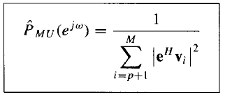
I am trying to use MUSIC algorithm to detect individual frequencies of an incident signal. I read the original paper and some interesting books that explain the algorithm. I used the following equation for estimating pseudospectrum.
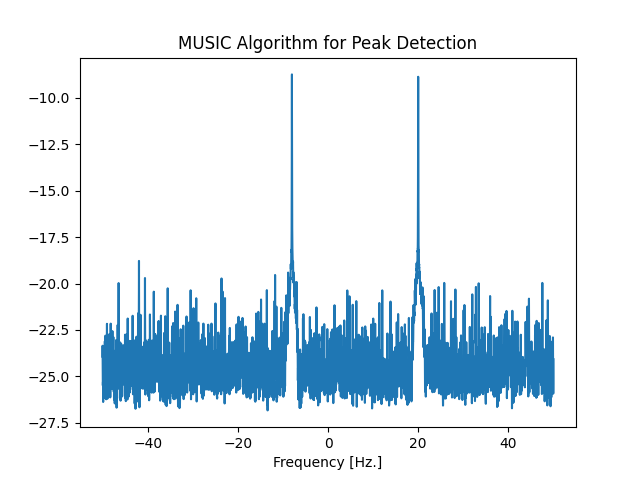
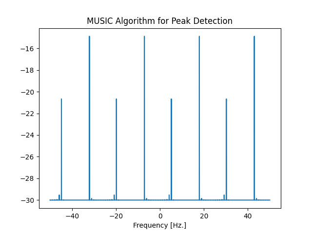
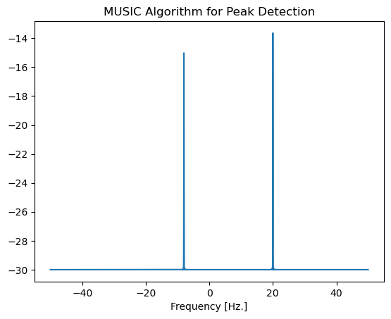
The above equation (Eq. 8.162) is given in Statistical Digital Signal Processing and Modelling book (by Monson Hayes). $\mathbf{v}_i$ is the eigenvectors of the noise subspace and $\mathbf{e}$ is the frequency vector. It is indicated that the term inside the summation in the denominator is equivalent to DFT of the noise subspace eigenvectors. Consequently, I implemented two different codes to estimate pseudospectrum using Eq. 8.162. The first code uses FFT of the eigenvectors and it works well, meanwhile the second code which uses exactly the same formula (without FFT) provides erroneous results. I hope if anyone can help me identify what is wrong in my implementation of that equation.
First code using FFT function
from scipy import signal
import numpy as np
from numpy import linalg as LA
from matplotlib import pyplot as plt
import scipy

N = 1000
nfft = 2**12

f1 = 20
f2 = -8
fs = 100

t=np.arange(0,N, 1)

c1 = np.exp(1j*2*np.pi*t*f1/fs)
c2 = np.exp(1j*2*np.pi*t*f2/fs)

snr = 10
stdev = 1/((10**(snr/10))**0.5)

data = c1 + c2 + 1/(np.sqrt(2)) * (stdev * np.random.normal(0, 1, N) + 1j * stdev * np.random.normal(0, 1, N))

p = 2
m = len(data)

# Develop autocorrelation matrix of the signal

acf = np.convolve(data,np.conj(data)[::-1])
center = int(np.ceil(len(acf)/2) - 1)
Rxx=acf[center:]
Rx = scipy.linalg.toeplitz(Rxx,np.hstack((Rxx[0], np.conj(Rxx[1:]))))

# Eigenvalue decomposition of the autocorrelation matrix

D, V = LA.eig(Rx)

# Sort the eigenvalues in ascending order

i = np.argsort(D)

# Estimate the summation

Px = 0

for index in range(0, m-p):
    Px = Px + np.abs(np.fft.fftshift(np.fft.fft(V[:, i[index]], nfft)))

Px = np.reciprocal(Px)
Px = 10*np.log10(Px)
w = np.arange(-fs/2, fs/2, fs/nfft)
plt.plot(w,Px)
plt.title('MUSIC Algorithm for Peak Detection')
plt.xlabel('Frequency [Hz.]')
plt.show()
The second code using Eq. 8.162
from scipy import signal
import numpy as np
from numpy import linalg as LA
from matplotlib import pyplot as plt
import scipy

N = 1000
nfft = 2**12

f1 = 20
f2 = -8
fs = 100

t=np.arange(0,N, 1)

c1 = np.exp(1j*2*np.pi*t*f1/fs)
c2 = np.exp(1j*2*np.pi*t*f2/fs)

snr = 10
stdev = 1/((10**(snr/10))**0.5)

data = c1 + c2 + 1/(np.sqrt(2)) * (stdev * np.random.normal(0, 1, N) + 1j * stdev * np.random.normal(0, 1, N))

p = 2
m = len(data)

# Develop autocorrelation matrix of the signal

acf = np.convolve(data,np.conj(data)[::-1])
center = int(np.ceil(len(acf)/2) - 1)
Rxx=acf[center:]
Rx = scipy.linalg.toeplitz(Rxx,np.hstack((Rxx[0], np.conj(Rxx[1:]))))

# Eigenvalue decomposition of the autocorrelation matrix

D, V = LA.eig(Rx)

# Sort the eigenvalues in ascending order

i = np.array(np.argsort(D))

freq_array = np.arange(-fs/2, fs/2, fs/nfft)
sum_array = np.zeros(nfft, dtype=np.float32)

print(np.shape(V[:, i[0]]))

for f in np.arange(0, nfft, 1):

    frequencyVector = np.zeros(m, dtype=np.complex_)

    for index in np.arange(0, m):
        frequencyVector[index] = np.exp(2 * np.pi * index * freq_array[f] * 1j)

    sum = 0
    for index in np.arange(0, m - p):
        sum = sum + np.abs(np.dot(np.transpose(np.conjugate(frequencyVector)), V[:, i[index]]))**2

    sum_array[f] = 10*np.log10(1/sum)

plt.plot(freq_array,sum_array)
plt.title('MUSIC Algorithm for Peak Detection')
plt.xlabel('Frequency [Hz.]')
plt.show()


