Taking The Inverse FFT And Extrapolating For Future Predictions In R

Question

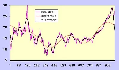
This is what I am trying to achieve:

See how the increasing number of harmonics are creating a good fit? I am trying to find the components of a given wave (discrete samples), and then to make brief prediction about where the curve is going from the generated cosines. Is it ok to use the inverse DFT and use the returned coefficients in a cosine statement? Here are the first few returned scalars from ifft:

8.142999e-01+0.00000e+00i 5.441907e-01+0.00000e+00i [3] 7.696127e-01-0.00000e+00i 7.745780e-01+0.00000e+00i [5] 9.672294e-01-0.00000e+00i 5.382324e-01-0.00000e+00i [7] 3.872890e-01-0.00000e+00i 5.561072e-01-0.00000e+00i

See these constants? I would like to use them like this:

Approximate wave = $a_o\cos(t) + a_1\cos(t) + a_2\cos(t) + a_3\cos(t) + \cdots$ where $a_i$ are the coefficients mentioned above.

The real constants are created using a cosine sum. See the $\cos(t)$ in every term? Does this make sense?

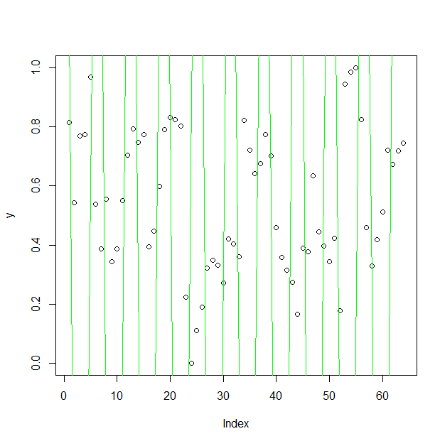
I have been using R and it looks to be getting somewhere when I use $0.8142999 * cos(t)$, the lowest fundamental.

This is getting somewhere, but I am obviously missing something. Please help.

Here Is My Code:

library(stats)
library(scales)

x <- c(0,1,2,3,4,5,6,7,8,9,10,11,12,13,14,15,16,17,18,19,20,21,22,23,24,25,26,27,28,29,30,31,32,33,34,35,36,37,38,39,40,41,42,43,44,45,46,47,48,49,50,51,52,53,54,55,56,57,58,59,60,61,62,63)
y <- c(0.86809,0.86537,0.86764,0.86769,0.86963,0.86531,0.86379,0.86549,0.86336,0.86378,0.86543,0.86699,0.86787,0.86742,0.86767,0.86386,0.86439,0.86591,0.86785,0.86826,0.8682,0.86797,0.86214,0.85989,0.86101,0.86181,0.86314,0.86339,0.86323,0.86263,0.86412,0.86396,0.86352,0.86816,0.86716,0.86634,0.8667,0.86767,0.86696,0.86452,0.86349,0.86307,0.86265,0.86155,0.8638,0.8637,0.86628,0.86437,0.86388,0.86335,0.86415,0.86169,0.86941,0.8698,0.86996,0.86819,0.86451,0.8632,0.86409,0.86504,0.86716,0.86667,0.86712,0.86739)
y <- rescale(y)

a <- fft(y, inverse=FALSE)
b <- fft(a, inverse=TRUE) /length(a)

t = seq(0, length(b) - 1, 1)

plot(y)

# constants from b
response = 8.142999e-01 * cos(t) + 5.441907e-01 * cos(t) + 7.696127e-01 * cos(t)
lines(x, response, col="green")

Answer 1

Have you read the source that your image comes from? It goes into details into the interpolation algorithm that you're trying to implement... Maybe start there? In particular:

Next I interpolate the data for the 90 days that the model is trying to predict, this is done by taking the Discrete Fourier Transformation with the equation form of:

a(k)=real(Y(k));
b(k)=-imag(Y(k));
omk=2*pi*(k-1)/365;
YY(n)=YY(n)+a(k)*cos(omk*(n-1))+b(k)*sin(omk*(n-1));a(k)=real(Y(k));

As a side-note: as interesting a use of the DFT this might be, I'm not sure I'd trust this method to do any reliable prediction. Might want to look at more machine learning based methods, especially if you're actually going to use this for financial decisions!