What is the cause of STFT artifacts when different signals overlap?

Question

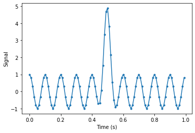
I'm trying to learn about why signals that cross in an STFT cause apparent artifacts in the magnitude. I've been looking at the example below, written in python, where a gaussian peak overlaps with a sinusoidal wave.

import numpy as np
from scipy import signal
import matplotlib.pyplot as plt

time = time = np.arange(0,1,0.01)

sine = np.cos(2*np.pi*10*time)
gaus = 4.0 * signal.windows.gaussian(time.shape[0],2)

plt.plot(time, sine + gaus, '.-')
plt.xlabel("Time (s)")
plt.ylabel("Signal")
plt.show()

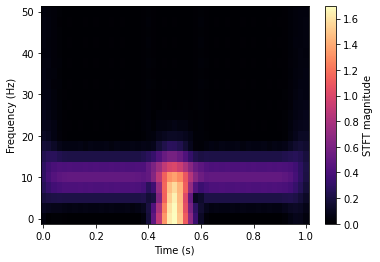
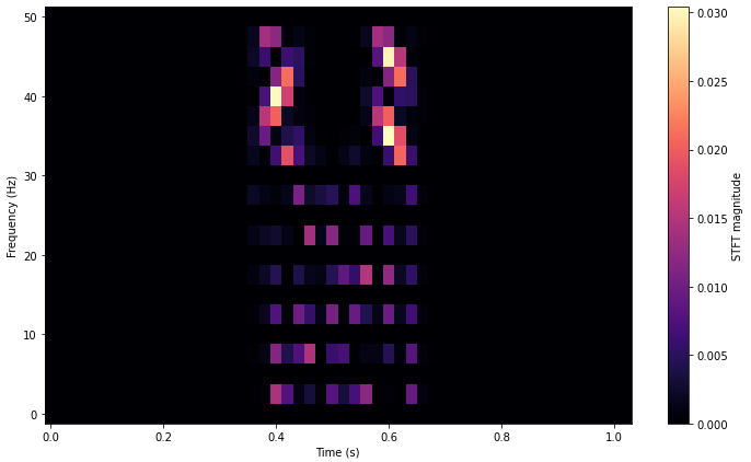
When I take the STFT of the signal and look at the magnitude of the output, there are some artifacts or edge effects near where the gaussian and sinusoidal signals overlap in time-frequency space. They appear as slight decreases in the magnitude.

fs = 100
window='hamming'
nperseg=20
noverlap=18
nfft = 2*nperseg

f,t,Zxx_sum = signal.stft(sine + gaus, fs=fs, window=window, nperseg=nperseg, \
                           noverlap=noverlap, nfft=nfft, return_onesided=True)

plt.pcolormesh(t,f,np.abs(Zxx_sum),cmap='magma')
plt.colorbar(label="STFT magnitude")
plt.xlabel("Time (s)")
plt.ylabel("Frequency (Hz)")
plt.show()

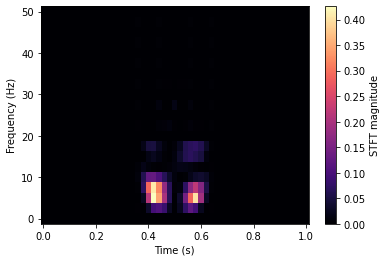
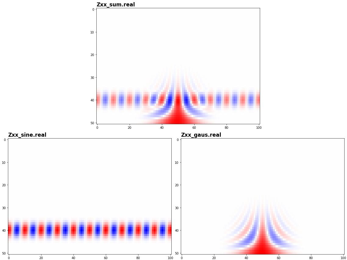
What is the origin of the slight decreases in the magnitude? Is this related to the window or the overlap? Why does the STFT magnitude of this signal not equal the sum of the magnitudes of the individual parts? I have plotted this below for clarity.

f,t,Zxx_sine = signal.stft(sine, fs=fs, window=window, nperseg=nperseg, \
                           noverlap=noverlap, nfft=nfft, return_onesided=True)
    
f,t,Zxx_gaus = signal.stft(gaus, fs=fs, window=window, nperseg=nperseg, \
                           noverlap=noverlap, nfft=nfft, return_onesided=True)
    
plt.pcolormesh(t,f,(np.abs(Zxx_sine) + np.abs(Zxx_gaus)) - np.abs(Zxx_sum),cmap='magma')
plt.colorbar(label="STFT magnitude")
plt.xlabel("Time (s)")
plt.ylabel("Frequency (Hz)")
plt.show()

Answer 1

Why does the STFT magnitude of this signal not equal the sum of the magnitudes of the individual parts?

Because magnitude, i.e. complex modulus, is a nonlinearity:

$$ |X| + |Y| = |a + jb| + |c + jd| \neq |X + Y| $$

and your $X$ and $Y$ are intersecting time-frequency geometries:

This isn't an artifact, it's consistent with STFT's interpretation as a Heisenberg-bound tool: the Gaussian "pulse"'s time-frequency geometry spans the entire plane, but is localized in (in your case) low frequencies, hence STFT sees an interference between that and the low-frequency pure tone which locally cancels (or amplifies) oscillations, hence removing their magnitudes. For a detailed treatment, see Peter K.'s reference.

To get the behavior you describe in approximation, un-intersect these geometries:

sine = np.cos(2*np.pi*40*time)

Note the colormap range; we can obtain float-equality with different parameters. Also for my convenience I used a different stft on the .real plots, but all results hold.

Answer 2

Fundamentally, it's about what I'd call cross-terms.

Here's an excruciatingly detailed example of deriving an analytic version of it for one particular case: where there are two complex exponential terms with frequencies $f_1$ and $f_2$. (Wish I still had the $\LaTeX$ for this so I could MathJAX it).

Reference:

Peter J. Kootsookos, Brian C. Lovell, Boualem Boashash, "A Unified Approach to the STFT, TFDs, and Instantaneous Frequency," IEEE Transactions on Signal Processing, vol. 40, no 8, August 1992, pp. 1971--1982. DOI: 10.1109/78.149998