A Butterworth filter is a a maximally flat, continuous time (analog) filter. That is it has the flattest passband possible, for a given cutoff frequency and filter order.
Frequency Response
The frequency response of a low-pass Butterworth filter is given by:
$$G^2(\omega) = |H(j\omega)|^2 = \frac{G_0^2}{1+\left(\frac{j\omega}{j\omega_c}\right)^{2n}}$$
where $G(\omega)$ is the gain as a function of the radian frequency ($\omega = 2\pi f$), $H(j\omega)$ the transfer function of the filter, $H(s)$ evaluated at $s = j\omega$, $G_0$ the DC gain (gain at zero frequency), $n$ the filter order, $\omega_c$ the cutoff frequency, and $j$ the imaginary unit.
Often filter prototypes are defined with $G_0 = 1$ and that will be assumed here.
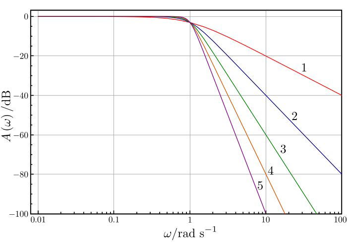
The cutoff frequency is the frequency at which the gain of the filter has been reduced by a factor of 2, approximately -3 dB ($10\log_{10}(1/2) \approx 3.01$).
The figure below is a plot of the frequency response for a lowpass Butterworth filter with order varying from 1 to 5 with $\omega_c = 1$.

Image from Wikipedia.
Transfer Function
The transfer function can be expressed as a ratio of a numerator polynomial and a denominator polynomial. For the low pass Butterworth filter the numerator is always $1$ and the denominator is a function of the filter order. For normalized cutoff, $\omega_c = 1$:
$$H(s) = \frac{1}{B_n(s)}$$
where for even $n$:
$$B_n(s) = \prod_{k=1}^{n/2} \left[s^2 - 2s\cos\left(\frac{2k+n-1}{2n}\pi\right)+1\right]$$
and for odd $n$:
$$B_n(s) = (s+1)\prod_{k=1}^{(n-1)/2} \left[s^2 - 2s\cos\left(\frac{2k+n-1}{2n}\pi\right)+1\right]$$
The first few value are
|n|$B_n$(s)|
|-|--------|
|1|$(s+1)$ |
|2|$(s^2 +\sqrt{2}s+1)$|
|3|$(s+1)(s^2+s+1)$|
Low-Pass to Band-Pass Transformation
Next, the prototype filter needs to be converted from low pass to band pass. Assuming a normalized prototype, $\omega_c = 1$, this can be achieve with a substitution of variables:
$$H(j\omega) \rightarrow H\left(Q\left[\frac{j\omega}{\omega_0} + \frac{\omega_0}{j\omega}\right]\right)$$
where $Q=\frac{\omega_0}{\Delta\omega}$, $\omega_0$ is the center of the bandpass passband, and $\Delta\omega$ is the bandwidth of the passband.
Conversion to Discrete Time (Digital)
According to the MATLAB documentation for the butter function, it uses the bilinear transformation with frequency prewarping to convert from continuous to discrete domain.
To provide a more faithful digital response, prewarping is applied to the cutoff frequencies of the band-pass filter (as it is bandpass there is a low and an upper cutoff). This would be done in the previous section when computing the frequency mapping to convert from low pass to bandpass.
The prewarping transformation is given by:
$$\omega_p=\frac{2}{T}\tan\frac{\omega_1 T}{2}$$
where $\omega_p$ is the prewarped cutoff frequency, $\omega_1$ is the corresponding cutoff frequency prior to prewarping, and $T$ is the sample period of the desired discrete time filter.
Finally, the bilinear transformation is applied to convert from continuous to discrete time:
$$s \rightarrow \frac{2(1-z^{-1})}{T(1+z^{-1})}$$
With this substitution made, the desired discrete time transfer function, $H(z)$, is arrived at.

