4
$\begingroup$

I implemented the plain DTF / inverse DFT algorithm in C++ in order to help me understand the method. As a sample input I considered

$$ f(x) = \sin \left( \tfrac{\pi}{5} x \right) $$

and collected samples for x = 0, ..., 9. So my input data was (0, 0.58778, 0.951057, ...).

Computing the DFT formula gives two non-zero coefficients: c_1 = (0 - 5i) and c_9 = (0 + 5i).

Now, I compute the inverse DFT. For x=1, these coefficients multiplied with their basis functions give

$$ \tfrac{1}{10} e^{i 2 \pi (1/10)} \cdot (0 - 5i) = (0.293893 -0.404508i) $$

and

$$ \tfrac{1}{10} e^{i 2 \pi (9/10)} \cdot (0 + 5i) = (0.293893 +0.404508i) $$

respectively which is correct as the real parts sum up to 0.58778 (thus, reconstructing the input value) and the imaginary parts sum up to 0. This works great for integral timestamps x=0, 1, 2, ...

My question: ... but how to interpret the results if I plug in x=0.5 (result 0.000000 - 0.951057i) or x=1.5 (result 0.000000 - 0.587785i) for example? I see that it is not DFT's promise to provide a good interpolation here. But is there an intuitive interpretation? (Came across this because I wanted to plot the DFT/IDFT result as a time-continuous graph and don't know how to deal with the complex results between)

EDIT

I add my C++ code here:

void dft( const std::vector<double> & vInput, std::vector< std::complex<double> > & vCoeff )
{
    const std::complex<double> i( 0., 1. );

    const int nElem = vInput.size();

    vCoeff = std::vector< std::complex<double> >( nElem, std::complex<double>(0., 0.) );

    for( int k = 0; k < nElem; ++k )
    {
        for( int j = 0; j < nElem; ++j )
        {
            vCoeff[k] += exp( -2. * M_PI * i * std::complex<double>( j, 0. ) * std::complex<double>( (double)k / nElem, 0. ) ) * vInput[j];
        }
    }
}
std::complex<double> inverseDft( const std::vector< std::complex<double> > & vCoeffs, const double t )
{
    std::complex<double> result( 0., 0. );
    const std::complex<double> i( 0, 1 );
    const int nElem = vCoeffs.size();

    for( int j = 0; j < nElem; ++j )
    {
        result += vCoeffs[j] * exp( 2. * M_PI * i * std::complex<double>( j, 0. ) * std::complex<double>( t / nElem, 0. ) );
    }

    return (result / nElem);
}

This is how I define my input:

std::vector<double> vInput;

for( int i = 0; i < 10; ++i )
{
    vInput.push_back ( sin( i * M_PI / 5 ) );
}

And this is the output I did not expect for t=0.5, t=1.5, etc.:

inverseDft( vCoeffs, 0. );  // okay (0.000000, -0.000000)
inverseDft( vCoeffs, 0.5 ); // ?? (0.000000, -0.951057)
inverseDft( vCoeffs, 1. );  // okay (0.587785, -0.000000)
inverseDft( vCoeffs, 1.5 ); // ?? (0.000000, -0.587785)

EDIT2

Great to have these expert answers here! I can contribute the 3D plot which supports my intuition and therefore might also be helpful for others. It shows f(t) computed by IDFT and how it travels over the original data points (crosses). In order to achieve this, it makes use of the whole space including the complex plane.

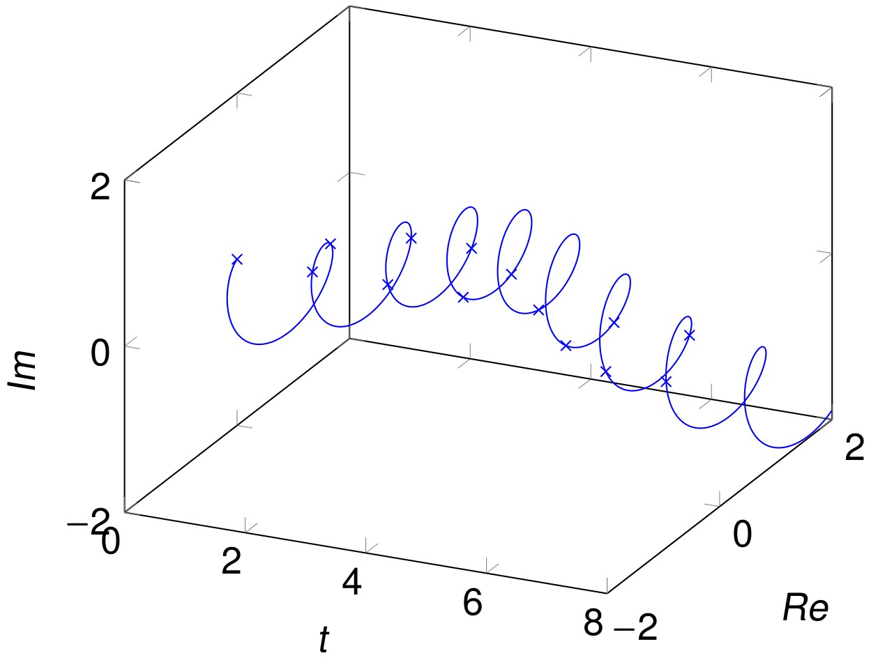
3D plot

$\endgroup$
1
  • 2
    $\begingroup$ i dunno what's intuitive but we've dabbled in this before in 1, 2, 3, 4 different times. i dunno if i have the energy to do it from scratch and rigorously. $\endgroup$ Commented Sep 26, 2020 at 1:30

3 Answers 3

4
$\begingroup$

The inverse DFT is

$$f[n] = \dfrac{1}{N} \sum_{k=0}^{N-1} F[k] e^{j2\pi\frac{k}{N}n}$$

You were computing

$$\begin{align*}g[n+d] &= \dfrac{1}{N} \sum_{k=0}^{N-1} F[k] e^{j2\pi\frac{k}{N}(n+d)}\\ \\ &= \dfrac{1}{N} \sum_{k=0}^{N-1} \left(F[k]e^{j2\pi\frac{k}{N}d}\right) e^{j2\pi\frac{k}{N}n}\\ \\ &= \mathrm{IDFT}\left\{F[k]e^{j2\pi\frac{d}{N}k}\right\}\\ \\ &= \mathrm{IDFT}\left\{F[k]\right\} \ast \mathrm{IDFT}\left\{e^{j2\pi\frac{d}{N}k}\right\}\\ \\ &= f[n] \ast \text{(a shifted sampled sinc() function with aliasing)} \\ \end{align*}$$

where $\ast$ denotes circular convolution.

The "shifted sampled sinc() function with aliasing" comes from taking the IDFT of a rectangularly windowed, frequency varying, exponential function.

The frequency varying exponential is the source of the shift.

The rectangular window (over the N points in the frequency domain), is the source of the sinc() function.

The limited time domain (N samples), trying to fit in the infinitely long sinc() function, manifests as aliasing.

The reason you don't notice this with shifts, $d$, that are an integer is that the sampled sinc() function looks like $[0, \dots, 0, 1, 0,\dots,0]$ for the case of an integer shift.

A "shifted sampled sinc() function with aliasing" is a horrible interpolation filter, as you may have noticed.

Update

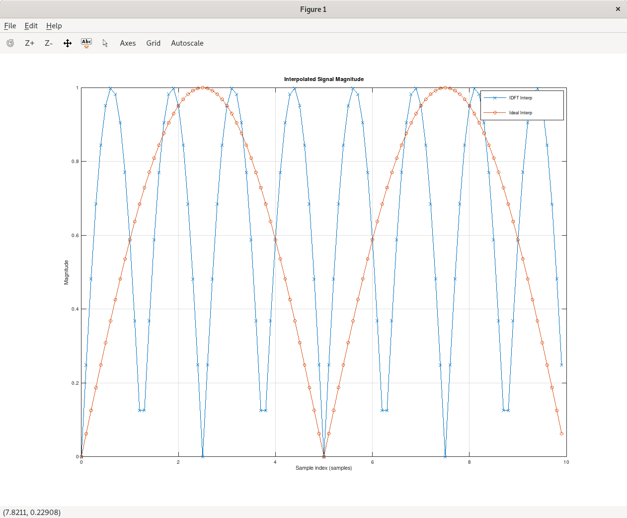
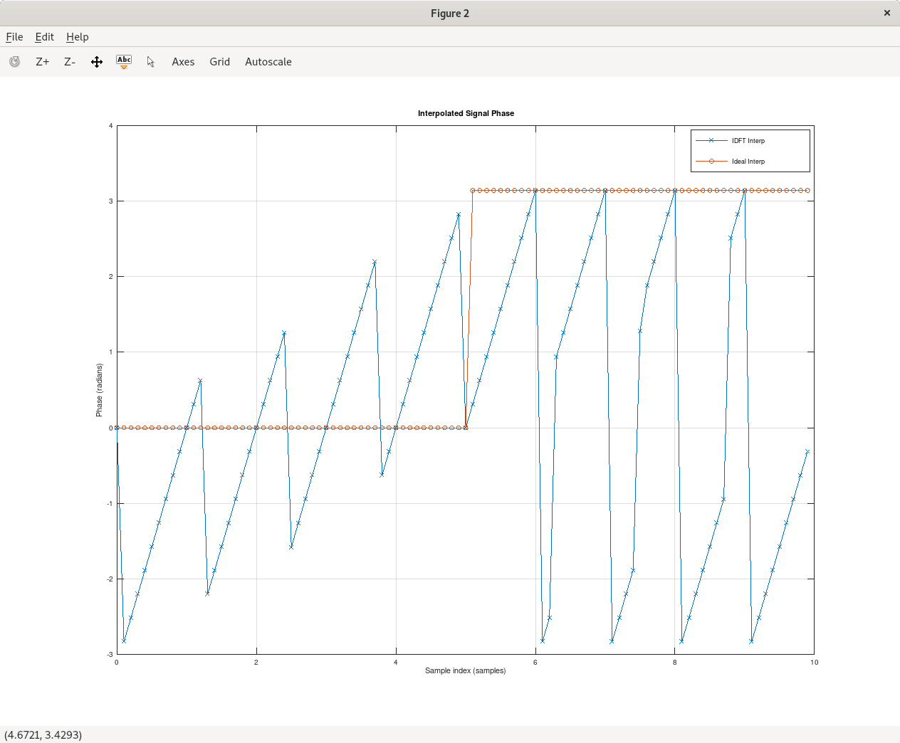
The following Octave (Matlab clone) script demonstrates the results of this "IDFT interpolation" technique to interpolate the original signal at intersample increments of $0.1$ samples:

N = 10;
x = [0:N-1];
f = sin(x*2*pi/N);
F = fft(f, N);

D = 10;
d = [0:D-1]/D;

x2 = ones(D,1)*x + d.'*ones(1,N);
F2 = ones(D,1)*F .* exp(1i*2*pi*d.'*ones(1,N)/N.*(ones(D,1)*x));
f2 = ifft(F2, N, 2);

x3 = reshape(x2, 1, D*N);
f3 = reshape(f2, 1, D*N);

fideal = sin(x3*2*pi/N);
figure(1);
plot(x3, abs(f3), 'x-;IDFT Interp;', x3, abs(fideal), 'o-;Ideal Interp;');
title('Interpolated Signal Magnitude');
xlabel('Sample index (samples)');
ylabel('Magnitude');
grid on;

figure(2);
plot(x3, arg(f3), 'x-;IDFT Interp;', x3, arg(fideal), 'o-;Ideal Interp;');
title('Interpolated Signal Phase');
xlabel('Sample index (samples)');
ylabel('Phase (radians)');
grid on;

Here are the output magnitude and phase plots of the "IDFT interpolated" signal vs. the ideal interpolated signal:

enter image description here

enter image description here

At integer sample indices, the magnitude and phase of the two signals exactly match, so the DFT and IDFT are correct. No surprise there.

At non-integer sample indices, the phase indicates the signal is complex valued, and the magnitude can be just as wrong as it could possible be, such as the values at sample index 2.5.

The magnitude of the the incorrect signal might be something like a 4x frequency sine wave of the original sine wave, but I don't know for sure. That relationship might just be a special case that happens because of the parameters picked in this particular example.

$\endgroup$
7
  • 1
    $\begingroup$ This is about the Dirichlet kernel, but I don't like the Wikipedia page on it. I will look for another, better, refefence. $\endgroup$ Commented Sep 25, 2020 at 17:46
  • $\begingroup$ @robertbristow-johnson Thanks. That looks more precise than my hand-waving at the end. I was drawing on experience from the DTFT/IDTFT. $\endgroup$
    – Andy Walls
    Commented Sep 25, 2020 at 17:49
  • $\begingroup$ @AndyWalls Thank you! I understand that interpolation can yield "horrible" results if (n+d) is not an integer. I am still not sure why IDFT is “hallucinating” these complex values between my real-valued input data. I am now guessing that if I plotted $f(n)$ from IDFT in 3D with continous time (like here), I would see some kind of "corkscrew" and in order to intersect the plane $Im=0$ when $n$ is an integer, it has to wiggle through the whole space. Is this right? $\endgroup$
    – Eddie C
    Commented Sep 25, 2020 at 19:09
  • $\begingroup$ Nice and correct answer for what is being asked. However, there's another possible interpretation of a slightly different inverse DFT with non-integer $n$, depending on how you construct your inverse DFT. That will yield a much better interpolation. Let me put an answer for that too. $\endgroup$
    – Fat32
    Commented Sep 25, 2020 at 19:25
  • $\begingroup$ @EddieC A real signal in the time domain transforms to a real-even + imaginary-odd function in the frequency domain. If you do something in the frequency domain to perturb that real-even + imaginary-odd configuration of the values, then you will end up with complex values in the time domain when performing the inverse transform. I'd really have to see your exact implementation to see what is going on. $\endgroup$
    – Andy Walls
    Commented Sep 25, 2020 at 20:04
5
$\begingroup$

Andy Walls provided the answer with the direct interpretation of an N-point inverse DFT with fractional time stamps. However, there is a slighty different (or totally should I've said) interpretation of a non-integer IDFT argument, which reduces to a good interpolation formula from the inverse DFT.

Consider the notation with $N,M,k,n$ being integers.

$$x_i[n] = \frac{1}{N} \sum_{k} X[k] \cdot e^{ j \frac{2\pi}{N} k (n) } \tag{0} $$

Lets say Eq.0 is a valid inverse DFT for some N-point $X[k]$, and results in a sequence $x_i[n]$, we ask what happens if we evaluate the sum at $n = n/M$; i.e., can we also plug $n/M$ into RHS $x_i[n]$ as given by Eq.1 below ?

$$x_i[n/M] = \frac{1}{N} \sum_{k} X[k] \cdot e^{ j \frac{2\pi}{N} k (n/M) } \tag{1} $$

Where $X[k]$ is the $N$-point DFT of some sequence $x[n]$, and $x_i[n]$ is the time sequence that result from the inverse transform evaluated at non-integer time indices. And the range of summation is deliberately left out.

With the index notation of $n/M$ what's implied is not very clear. Plugging $n/M$ into an inverse DFT is formally not allowed as the argument $n/M$ is meaningless for the time-domain sequence. Yet it's possible to interpret the notation as an indicator of an oversampling of the implied interpolation applied on the $x[n]$ sequence.

In that sense, I would re-write the inverse DFT as $$x_i[n] = \frac{M}{L} \sum_{k} X[k] \cdot e^{ j \frac{2\pi}{N*M} k n } \tag{2}$$

Now $x_i[n]$ looks like an $L = M \times N$ point inverse DFT of the N-point forward DFT $X[k]$ of $x[n]$. But there're two alternative interpretations; the first one is explained by Andy Walls, in which the inverse DFT is applied to the zero appended DFT $X[k]$ which looks like:

$$x_i[n] = \frac{M}{L} \sum_{k=0}^{L-1} X[k] \cdot e^{ j \frac{2\pi}{L} k n } = \frac{M}{L} \sum_{k=0}^{N-1} X[k] \cdot e^{ j \frac{2\pi}{L} k n } \tag{3}$$

Using Matlab you can implement Eq.3 as:

xi = M*ifft( fft(x,N), L );

This is a terrible interpolation, as explained in the other answer.

But I would call it terrible because of the miss-placed zeros in the inverse DFT formula. It performs zero padding by appending zeros to the tail of $X[N-1]$ until the end $k=L-1$

Now, the other alternative is to add the zeros into the middle of $X[k]$, with the following associated inverse DFT, for $N$ even :

$$x_i[n] = \frac{M}{L} \big( \sum_{k=0}^{N/2} X[k] \cdot e^{ j \frac{2\pi}{L} k n } +\sum_{k=N/2+1}^{L-N/2} 0 \cdot e^{ j \frac{2\pi}{L} k n } + \sum_{k=L+1-N/2}^{L-1} X[k] \cdot e^{ j \frac{2\pi}{L} k n } \big) \tag{4}$$

In Eq.4, the orignal $N$-point DFT $X[k]$ is repeated $M$ times, (indicator of expanding $x[n]$ by $M$), and windowed by an $N$ point rectangular window with a symmetric placement (representing the frequency domain effect of an ideal lowpass brickwall filter applied on the expanded time-domain sequence), and then an L-point inverse DFT is performed to get the $L$-point interpolated sequence $x_i[n]$. This can be achieved in MATLAB with the following line :

xif = M*real(ifft([X(1:N/2+1), zeros(1,L-N),X(N/2+2:N)],L));

Now this is a quite good interpolator of $x[n]$ at a rate of $M$ times oversampling it...

$\endgroup$
1
  • 2
    $\begingroup$ Nice thinking outside of the box (of N points). $\endgroup$
    – Andy Walls
    Commented Sep 25, 2020 at 20:22
2
$\begingroup$

Without derivation, I am just gonna plop the result here:

If a "sufficiently" bandlimited, periodic, continuous-time signal, $x(t)$, is sampled (let's define our sampling period to be $T=1$, it's just a matter of choosing the unit of time):

$$ x[n] = x(nT) = x(n) \qquad \forall n\in\mathbb{Z} $$

And if the period is $N$:

$$ x[n+N] = x[n] \qquad \forall n\in\mathbb{Z} $$

Then the reconstructed continuous-time signal is (from the sampling and reconstruction theorem):

$$x(t) = \sum_{n=-\infty}^{\infty} x[n] \, \operatorname{sinc}(t-n),$$

where

$$ \operatorname{sinc}(u) \triangleq \begin{cases} \dfrac{\sin(\pi u)}{\pi u} & \text{if } u \ne 0, \\\;1 & \text{if } u = 0. \end{cases} $$

That can be rearranged:

$$\begin{align} x(t) &= \sum_{n=-\infty}^{\infty} x[n] \, \operatorname{sinc}(t-n) \\ &= \sum_{m=-\infty}^{\infty} \sum_{n=0}^{N-1} x[n+mN] \, \operatorname{sinc}\big(t - (n+mN)\big) \\ &= \sum_{m=-\infty}^{\infty} \sum_{n=0}^{N-1} x[n] \, \operatorname{sinc}\big(t - (n+mN)\big) \\ &= \sum_{n=0}^{N-1} \left(x[n] \, \sum_{m=-\infty}^{\infty} \operatorname{sinc}\big(t - n - mN \big)\right). \\ \end{align}$$

Substituting $u \triangleq t-n$ gives

$$ x(t) = \sum_{n=0}^{N-1} x[n] \, g(t-n), $$

where

$$ g(u) = \sum_{m=-\infty}^{\infty} \operatorname{sinc}(u-mN) $$

Clearly the continuous (and real) $g(u)$ is periodic with period $N$:

$$ g(u+N) = g(u) \qquad \forall u \in \mathbb{R} $$

For $N$ odd, it's the same as the Dirichlet kernel:

$$ g(u) = \frac{\sin(\pi u)}{N \sin(\pi u/N)} $$

For $N$ even, it's a little different:

$$ g(u) = \frac{\sin(\pi u)}{N \tan(\pi u/N)} $$

$\endgroup$

Your Answer

By clicking “Post Your Answer”, you agree to our terms of service and acknowledge you have read our privacy policy.

Not the answer you're looking for? Browse other questions tagged or ask your own question.