What is the impulse response used in an interpolation filter when upsampling?

Question

I need to downsample a single period waveform from $M$ samples to $L$ samples. If that matters, in my particular case, $L=M-1$.

I read about downsampling and came to the conclusion I need:

1. expand the original waveform by a factor $L$ (some other source call the step “zero stuffing”),
2. interpolate the missing samples,
3. decimate by a factor of $M$:

If I understood it correctly, expansion only requires adding $L-1$ zeros between each original sample. Decimation seems simple too since it only requires keeping every $M^{th}$ samples.

But I'm stuck with the interpolation process. The naive solution of using linear interpolation gave me surprisingly good results at low frequencies but quickly degraded when the frequency increases (i.e., .when the number of samples in the waveform decrease).

I found several mentions of using an interpolation filter that looks like a dot product¹. For example, on the Upsampling Wikipedia page, I see:

$$y[j+nL] = \sum_{k=0}^K x[n-k]\cdot h[j+kL],\ \ j = 0,1,\ldots,L-1,$$

where the h[•] sequence is the impulse response, and K is the largest value of k for which h[j + kL] is non-zero

In my understanding, $x[•]$ is the sequence after the expansion step. $y[•]$ is the upsampled waveform. But I don't understand what are $h[•]$ and $K$. I read they are related to the impulse response and I understand the concept. But I can't see where it comes from and how to obtain it in practice.

Could someone explain to me how to obtain $h[•]$ and $K$?

---

_{¹It also looks like a convolution to me, but I'm not quite sure of that. And apparently this would be an instance of FIR filter. We already talked about that in other questions, but this is still not clear to me.}

Answer 1

The dot in that summation is just scalar multiplication. And yes, it's a convolution -- you're convolving the input signal by the filter.

Answer 2

Below shows design considerations for the filter design and you can use common tools in Matlab/Octave and Python Scipy.Signal to determine the filter coefficients (impulse response) using this criteria. (such as the firls and firpm filter design commands in Matlab).

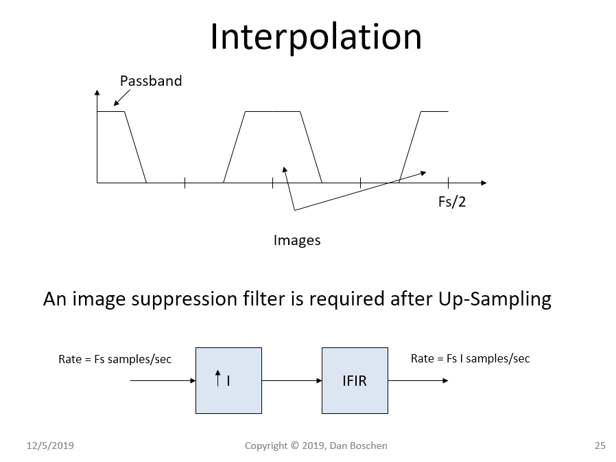
When you insert zeros, you create replicas in frequency such as I show in the diagram below, but beyond the replicas that exist at other frequencies, it does not distort your original band-limited spectrum. Therefore the ideal interpolator filter would pass your original spectrum without distortion and filter the replicas at the other frequencies completely. Any filter that could do this would give you ideal interpolation. (The reality is that no filter can achieve this, so we make compromises and design to achievable signal to noise ratios and other metrics for allowable distortion.)

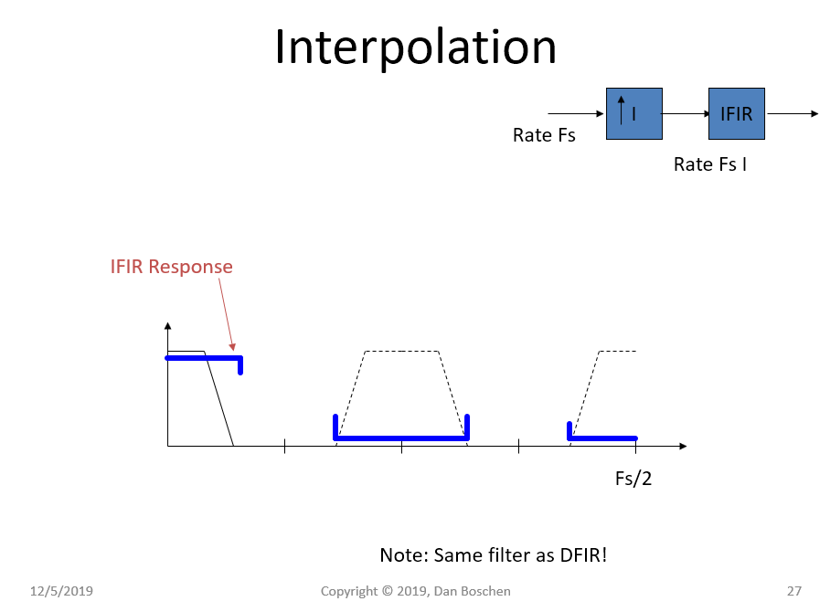
Your ability to approach the ideal filter will drive the complexity of the filter design. Note that since the replicas are in defined frequency locations (not over an entire stop-band of a typical low-pass filter), you can use multi-band filter design for a better interpolation filter given the same number of taps (Matlab, Octave, Python Scipy.Signal all have the ability to easily provide design solutions for multi-band filters and for that for this purpose I recommend the least-square filter alogorithm (see command firls in Matlab/Octave for further info on that).

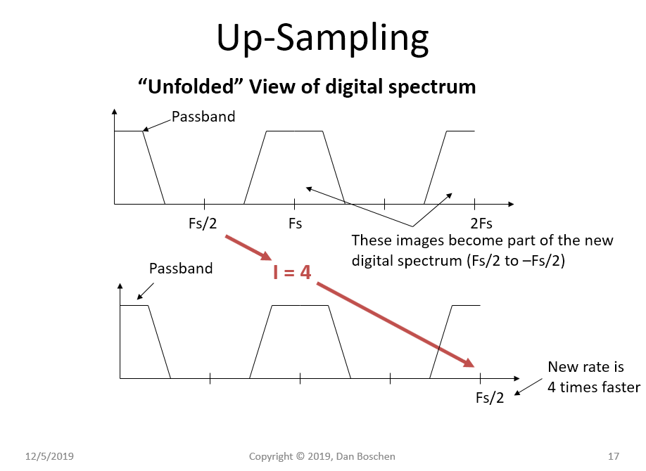
Below shows a simple example of an interpolate by 4 and the required filter design.

First let me explain the "unfolded" digital spectrum: If you allow the frequency axis of the sampled signal to extend to $\pm \infty$, instead of limiting to the unique digital frequency range of $\pm F_s/2$ (where $F_s$ is the sampling rate), you will see replicas of the original spectrum that is centered about 0 (DC) to also be similarly centered around every multiple of $F_s$. This is because the frequency axis is periodic for discrete time signals, which is why we only need to show the spectrum from $\pm F_s/2$ (or even $0$ to $F_s/2$ for real signals) since this replicates everywhere else. However, I find this visualization helps immensely in understanding many concepts in multi-rate signal processing as well as bridging analog and digital systems.

When we insert $N-1$ zeros (in the example diagram below $N=4$), this causes the sampling rate to increase N times but the images that exist around each multiple of the original sampling rate remain in their original positions. So in our new digital frequency span with the new $F_s$ that is $N$ times higher, we still have our original spectrum with no distortion within its spectral occupancy, but we have distortion as evidenced by the new images that are now part of our primary signal that exists in the new $\pm F_s/2$. So our ideal filter will not distort our primary signal of interest while reject these higher frequency images.

We could use a traditional low pass filter to simply pass our signal of interest and reject all higher frequencies, but common digital filter design algorithms (such as firpm and firls in Matlab, resulting in designs using the Parks-McLellan algorithm and Least Squares algorithm respectively) readily allow for multiband filter designs, which would concentrate the required rejection only where we need it. Below shows the target pass band and rejection bands we would use as a multiband filter design for this example.

As for your case, you may achieve better results by doing it in stages if you are able to factor L or M. This would be clearer once you see the filter design requirements given your ratios and your signal bandwidth.

See this post for another example of an interpolator filter design and its result:

Downsample: resample vs antialias fitlering + decimation