high & low pass correlated dither noise question

Question

I read a pretty cool article the other day: Robert Katz - Dither noise Probability Density Explained.

It says that if you have two dice (A and B) that you can roll both dice and then...

1. Re-roll die A and sum A and B

2. Re-roll die B and sum A and B

3. Re-roll die A and sum A and B

4. repeat to get a low pass filtered triangular noise distribution.

It says that you can modify it for high pass filtered triangle noise by rolling both dice and then...

1. Re-roll die A and take A - B

2. Re-roll die B and take B - A

3. Re-roll die A and take A - B

4. repeat to get a high pass filtered triangular noise distribution.

What i'm wondering is, what is the right thing to do if you want to do this with more than 2 dice? (going higher order)

For low pass filtered noise with 3+ more dice (which would be more gaussian distributed than triangle), would you only re-roll one die each time, or would you re-roll all BUT one die each time.

I have the same question about the high pass filtered noise with 3+ more dice, but in that case I think i know what to do about the subtraction order... I think the right thing to do if you have N dice is to sum them all up, but after each "roll" you flip the sign of every die.

Can anyone illuminate the correct way to do this?

Edit: I'm looking to get high and low pass filtering with more dice, but am fine with the distribution changing from triangle to gaussian or other shapes.

Answer 1

To achieve high-pass shaping , the “DC term” must be 0. Note that in the 2-dice high-pass case, every roll appears twice, once with a positive sign and once with a negative sign, which enforces the DC-free condition. Any scheme involving more than 2 dice would still need to meet this condition. The triangular PDF condition is satisfied by the fact that each sum or difference combines 2 rectangular PDF’s. I don’t know how you can get a triangular PDF by combining 3 rectangular PDF’s, regardless of how they are weighted.

Bob Adams

Answer 2

As stated with the die rolled sequentially (and assuming statistically identical dice) then it really makes no difference how many are used since we are operating on sequential rolls to compute each new output sample: you could do the same experiment with one die and just keep rerolling it to compute the next output by either subtracting (for high pass) or adding (for low pass) with the previous roll.

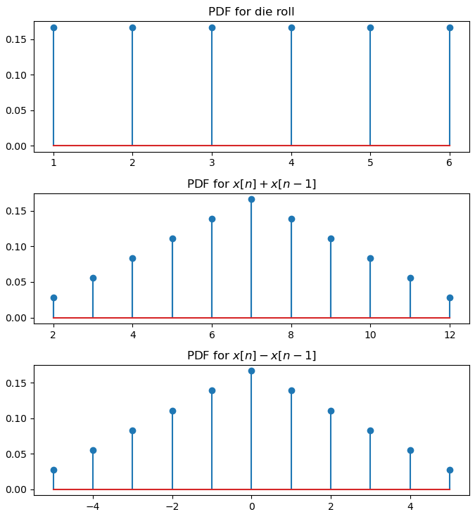
Each die roll is a random process with an independent uniform distribution (uniformly distributed over the 6 quantized values, assuming an unbiased die) - so if we choose on any subsequent roll to use the same die or different die, that doesn't change the statistical outcome of the experiment. This process is the sum of two independent random variables, in which case the probability distribution functions will convolve. The convolution of samples of a uniform distribution will result in samples of a triangular distribution as noted.

The random process with a roll of a die is ergodic which means the outcomes from the random variable given by rolling one die sequentially N times will be the same (in distribution and likelihood) as rolling N dice and using their outcomes as a sequential result. Therefore we can take the difference or sum of sequential outcomes from the same die or any number of different die with no change in the statistical properties of the result.

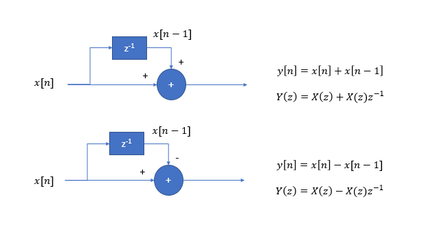
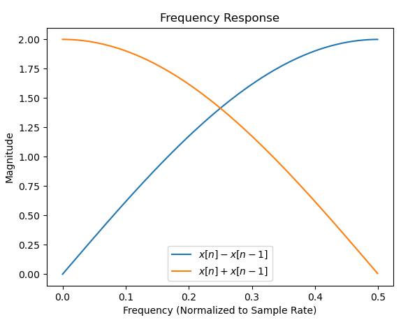
As far as the frequency response, this process is identical a two-tap FIR filter with the frequency transfer functions derived from the z-transform directly as shown in the diagram below with the unit circle as $z= e^{j\omega}$ with $\omega \in [0, 2\pi)$. And we see in the statistical characterization of the process that we have two unrelated characteristics, the probability distribution which shows us how often each event will occur (over all time) and the frequency response tells us how fast and how far the process can change from sample to sample with high frequencies favoring large sample to sample deviations and lower frequencies having less deviation from sample to sample:

Thus the summation as a low pass filter has the frequency response:

$$H(z = e^{j\omega}) = \frac{Y(z)}{X(z)} = \frac{1}{1+z^{-1}}$$

And the subtraction as a high pass filter has the response given by

$$H(z = e^{j\omega}) = \frac{Y(z)}{X(z)} = \frac{1}{1-z^{-1}}$$

Incidentally this is also the result of a 2 point DFT which is as two frequency bins the result of a low pass and high pass process.

Below I use the freqz function available in Matlab, Octave, and Python scipy.signal to show the magnitude response for both of these functions over the range from DC ($f=0$) to half the sampling rate where we clearly see the high pass and low pass result.

And for each case the resulting probability distribution functions would be the convolution of the two input (and independent) uniformly distributed functions:

The OP may have incorrectly assumed that increasing the number of die would approach a Gaussian distribution; this is clearly not the case if the die are still rolled sequentially, or more specifically if the process is still subtracting one die from any other to compute each new output sample. Doing that, as we described, has not changed the experiment as basically the moving average of 2 over all the rolls (a scaled average since we haven't divided by two) that we have shown above.

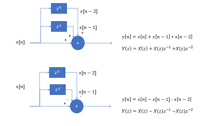
However, following the logic laid out above, we can see an example of what would occur in an actual higher order process and how that would be constructed and analyzed in terms of both the frequency response and the distribution. Consider this three sample process where we add all samples (in this case independent rolls of a die), or subtract the two subsequent samples from the first. Each $z^{-1}$ represents a 1 sample delay, so $z^{-2}$ is a 2 sample delay. Typically this would be drawn by cascading two $z^{-1}$ blocks, but I drew the block diagrams in this way to be most intuitive to the reader less familiar with FIR filters:

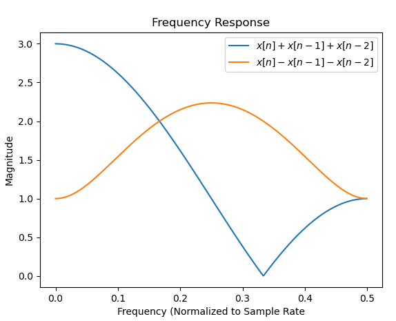
We can change the summations and subtractions to any of the 8 combinations resulting in eight different frequency responses (+++, ++-, +-+, +--, -++, -+-, --+, ---). The magnitude response of some of these will be the same but in terms of magnitude and phase, each response would be unique. The updated block diagram above shows the +++ and +-- combination. The frequency response magnitude for these two cases would be as shown in the figure below:

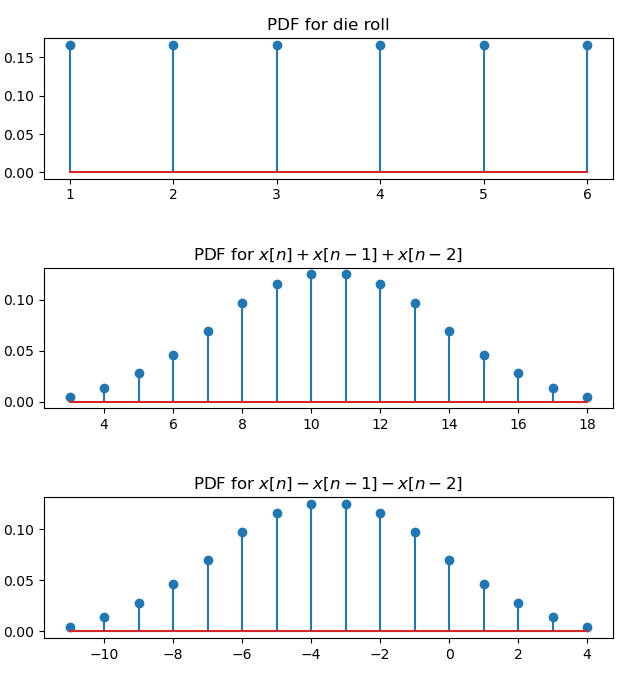
The pdf of the resulting random process given by each output sample (as the sum of three input samples) is the convolution of the pdf of the random process given by the inputs. Here as above the inputs are samples of a uniform distribution, and as the OP suspected, in THIS case the result will begin to approach a Gaussian (this is actually significantly off from a true Gaussian but we can start to recognize what is occurring due to the convolution- once we get above summing 6 or 7 samples the deviation from a Gaussian becomes quite small for most applications and ultimately we are seeing the result of the Central Limit Theorem at play). As above, the convolution in all cases does not change the shape of the distribution (a sum or a subtract is still a summation when the input is an independent random variable, changing it's sign does not change how the two are inter-related), but it does change the range of the output. This is intuitive, if you roll three die and sum the result, the range will be 3 to 18. But if you roll three die and subtract two from the first, the range is -11 to 4.

We see here a succinct distinction when considering the properties of random variables: We are interested in their frequency content and the distribution of their values- these are two different properties that are independent of each other (I find many confuse a Gaussian process as having a Gaussian distribution in frequency, but "Gaussian" is the distribution of the magnitude. We need to further clarify if the process is white to indicate all frequencies are present (as would be for a process that is independent from sample to sample since we can get any deviation from sample to sample), or if the process is low-pass or high-pass, for example.