Frequency estimation on chaotic waveform

Question

The target signal is generated by the following analytically solvable hybrid chaotic oscillator

\begin{equation}\label{eq:1} \ddot{u} - 2\beta \dot{u} +(\omega^2+\beta^2)(u-s)=0 \end{equation}

where

• $\omega$ determines the symbol period as $T = \frac{2\pi}{\omega}$.

• $\beta \in (0,T^{-1}\ln 2)$ affects the fluctuating amplitude.

• $s \in{\pm 1}$ is the random bipolar symbol sequence driving the system.

Its typical continuous waveform $u(t)$ for $f=100 \, \mathrm{Hz}$ is as follows:

I am interested in estimating the basis frequency $f$ of the signal. However, the amplitude spectrum of $u(t)$ has no obvious feature that can be used to estimate the frequency. Hence, I calculate

$$z(t) = |u(t)| - 1$$

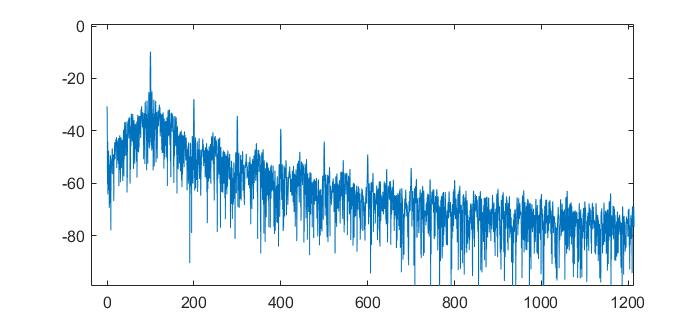
The amplitude spectrum of $z(t)$ is as follows

Obviously, we can see a spike at $f = 100 \, \mathrm{Hz}$. But it is hard to calculate the accurate expression of $z(f)$ since $u(t)$ is a kind of non-stationary signal.

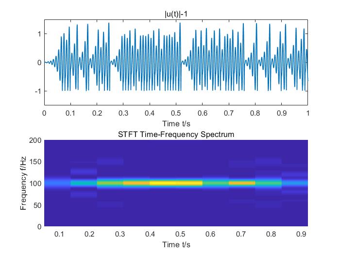
The STFT time-frequency spectrum is shown below

As shown in the STFT results, in some time intervals, no obvious frequency component can be found. However, in the part of approximately periodic waveform, the frequency component at $f = 100 \, \mathrm{Hz}$ is strong.

Is there any theory that can support my method of frequency estimation from the FFT of the whole $z(t)$?

---

Here is the MATLAB code for generating the chaotic waveform from an analytical expression (not provided above) and my current experiments on frequency estimation.

clear;close all;

finit = 100;%set frequency
% finit =2000;
% finit =2;
om=2*pi*finit;
be=om/(2*pi)*log(2)-0.01*rand(1,1);
T = 2*pi/om; %Period
N=100;% number of symbol
tall = N*T;%total time
h=T*0.01;%time step
t=0:h:tall-h;
ut=zeros(1,length(t));
u_in = 2*rand(1)-1;
% u_in =0.99;
for i=1:N
    if u_in>=0
        s_in = 1;
    else
        s_in = -1;
    end
    t_f = (i-1)*T:h:i*T-h;  %Time of each frame
    n_f = (i-1)*length(t_f)+1:i*length(t_f);
    ut(n_f)=s_in+(u_in-s_in)*exp(be*(t_f+(1-i)*T)).*...
           (cos(om*t_f)-be/om*sin(om*t_f));
    u_in=s_in+(u_in-s_in)*exp(be*T)*cos(om*i*T);
end

figure
plot(t, ut)
xlabel('Time t/s');
title('u(t)')

y = abs(ut) - 1; % Observed signal

%% FFT spectrum
L = length(ut);
Ts_v = t./(0:L-1);
Fs = ceil(1/Ts_v(2));
deltaf= 0.1;
NFFT = floor(Fs/deltaf);
fs = Fs;
f = Fs/2*linspace(0,1,floor(NFFT/2+1));
Y = fft(y,NFFT)/L;
Yabs = 20*log10(abs(Y(1:floor(NFFT/2+1))));
figure;
plot(f,Yabs);
xlim([0,max(f)/4]);
ylim([-100,0]);
xlabel('Frequency f/Hz');
title('FFT Spectrum');
%%  Wavelet Transfrom Time-Frequency spectrum
wavename='cmor3-3';
totalscal=256*2;
Fc=centfrq(wavename); 
c=2*Fc*totalscal;
scals=c./(1:totalscal);
f=scal2frq(scals,wavename,1/fs); 
coefs=cwt(y ,scals,wavename); 


figure;
subplot(211)
plot(t,y,'linewidth',1)
xlim([0 1])
ylim([-1.5 1.5])
subplot(212)
imagesc(t,f,abs(coefs));
set(gca,'YDir','normal')
ylim([0 200]);
% colorbar;
xlabel('Time t/s');
ylabel('Frequency f/Hz');
title('Wavelet Time-Frequency Spectrum');
%% STFT Time-Frequency spectrum
window_len = 10*2*pi/om/h;
noverlap = 50;
nfft = NFFT;
[~,F,T,P]=spectrogram(y,hamming(window_len),noverlap,nfft,fs);


figure;
subplot(211)
plot(t,y,'linewidth',1)
xlabel('Time t/s');
title('|u(t)|-1')
xlim([0 1])
ylim([-1.5 1.5])
subplot(212)
surf(T,F,abs(P),'edgecolor','none')
axis tight;
view(0,90)
ylim([0 200]);
xlabel('Time t/s');
ylabel('Frequency f/Hz');
title('STFT Time-Frequency Spectrum');
```

Answer 1

Here is a stab.

Start with:

$$ \ddot{u} - 2\beta \dot{u} +(\omega^2+\beta^2)(u-s)=0 $$

Take the derivative:

$$ \dddot{u} - 2\beta \ddot{u} +(\omega^2+\beta^2)(\dot{u}-\dot{s})=0 $$

Now, $ \dot{s} = 0 $ Wherever it is defined. So:

$$ \dddot{u} - 2\beta \ddot{u} +(\omega^2+\beta^2)(\dot{u})=0 $$

Let $ v = \dot{u} $, and you get

$$ \ddot{v} - 2\beta \dot{v} +(\omega^2+\beta^2)v=0 $$

Which is an ordinary second degree linear differential equation. v will have the same frequency as u.

The most basic (good) differential approximation is:

$$ d[n] = \frac{u[n+1]-u[n-1]}{2} $$

So run that over your data and see what you get and please add a chart to your question with the results.

I think you may best solve this one by analyzing the zero crossing of those results. The transitions are going to cause weirdness as your system "falls" towards the new equilibrium.

---

Followup:

A more traditional approach perhaps.

$$ \ddot{u} - 2\beta \dot{u} +(\omega^2+\beta^2)(u-s)=0 $$

Your homogenuous equation is:

$$ \ddot{u} - 2\beta \dot{u} +(\omega^2+\beta^2) u=0 $$

with solutions:

$$ u_h = \left[ C_1 \cos( \omega t ) + C_2 \sin( \omega t ) \right] e ^ { \beta t } $$

And your particular equation is:

$$ \ddot{u} - 2\beta \dot{u} +(\omega^2+\beta^2) s=0 $$

Assume:

$$ u = a t^2 + b t + c $$

$$ \dot{u} = 2 a t + b $$

$$ \ddot{u} = 2 a $$

$$ (2a) - 2\beta ( 2 a t + b ) + (\omega^2+\beta^2) s=0 $$

$$ (2 - 4 \beta t) a - 2\beta b + (\omega^2+\beta^2) s=0 $$

$$ a = 0 $$

$$ b = \frac{\omega^2+\beta^2}{2\beta} \cdot s $$

So :

$$ u_p = \left( \frac{\omega^2+\beta^2}{2\beta} \cdot s \right) t $$

For any range of consistent $s$ you now have your general and particular solutions.

Therefore you should only need five points to solve for your five unknowns: $ \omega, \beta, C_1, C_2,$ and $ c $.

With noise, that goes out the window. If you take the second derivative, your particular solution will be squashed completely. Then you should only have to worry about the $s$ transition points.

Line crossings will give you $\omega$, and the envelope will give you $\beta$.