Ratio of expected values of squares of errors in power quantities, in dB

Question

An amplitude quantity $a$ is estimated by two estimators $\hat a_1$ and $\hat a_2.$ The error of estimator $\hat a_2$ is compared to that of $\hat a_1$. One possible comparison is the ratio of expected values of absolute error:

$$\frac{\operatorname{E}[|a - \hat a_2|]}{\operatorname{E}[|a - \hat a_1|]}.$$

This is a ratio of amplitude quantitities and can be expressed in decibels as:

$$20 \log_{10}\left(\frac{\operatorname{E}[|a - \hat a_2|]}{\operatorname{E}[|a - \hat a_1|]}\right) \text{ dB.}$$

Another possible comparison is the ratio of expected values of square error:

$$\frac{\operatorname{E}[(a - \hat a_2)^2]}{\operatorname{E}[(a - \hat a_1)^2]}.$$

This is a ratio of power quantities and can be expressed in decibels as:

$$10 \log_{10}\left(\frac{\operatorname{E}[(a - \hat a_2)^2]}{\operatorname{E}[(a - \hat a_1)^2]}\right) \text{ dB.}$$

The squares of the estimators can be used to estimate $a^2.$ The estimators $\hat a_1^2$ and $\hat a_2^2$ can be compared by the ratio of expected values of square error:

$$\frac{\operatorname{E}[(a^2 - \hat a_2^2)^2]}{\operatorname{E}[(a^2 - \hat a_1^2)^2]}.$$

This is a ratio of squares of power quantities. How should it be expressed in decibels?

$$10 \log_{10}\left(\frac{\operatorname{E}[(a^2 - \hat a_2^2)^2]}{\operatorname{E}[(a^2 - \hat a_1^2)^2]}\right) \text{ dB,}$$

or perhaps:

$$5 \log_{10}\left(\frac{\operatorname{E}[(a^2 - \hat a_2^2)^2]}{\operatorname{E}[(a^2 - \hat a_1^2)^2]}\right) \text{ dB} = 10 \log_{10}\left(\frac{\sqrt{\operatorname{E}[(a^2 - \hat a_2^2)^2]}}{\sqrt{\operatorname{E}[(a^2 - \hat a_1^2)^2]}}\right) \text{ dB},$$

where the square roots are power quantities, or is there no commonly agreed convention?

Answer 1

Your question raises many very present concerns about measuring differences, and optimizing, in signal/image processing. Measuring can help:

• to compare different outcomes from two different processes,
• to optimize processing per se (for denoising, restoration).

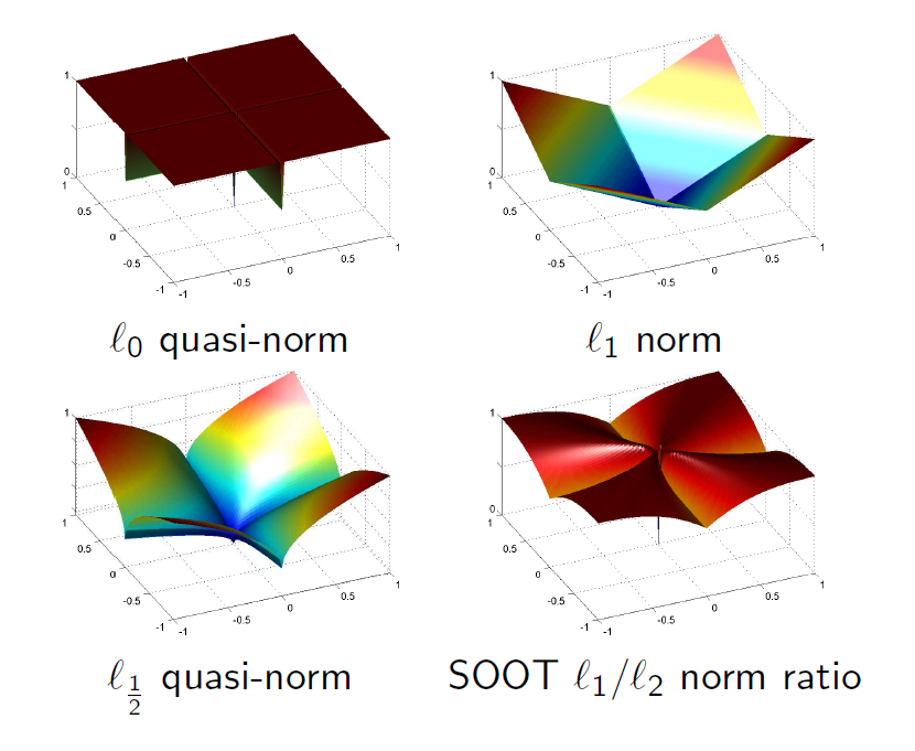
Most use cost functions related to $p$-norms (when $p\ge 1$) or quasi-norms (when $0<p\le 1$): $$\mathcal{C}_p(a,\hat{a})=\left(\sum_k|a_k-\hat{a}_k|^p\right)^{1/p}\,.$$ Those functions are symmetric, and are consistent with the physical units of $a$. The behavior of $\mathcal{C}_p$ depends on power $p$: classical norm inequalities tells you that $\mathcal{C}_p(a,\hat{a})\ge \mathcal{C}_q(a,\hat{a})$ when $p\le q$. Those (quasi-)norms are $1$-homogeneous. Using different $p$ or $q$ can be useful, especially in a sparsity context, see for instance references in: Euclid in a Taxicab: Sparse Blind Deconvolution with Smoothed \ell_1/\ell_2 Regularization. Here is a rendition of classical penalties:

Thus, quasi-norm or norm ratios are used to compare estimates, in a unitless fashion. The $\ell_p$ signal-to-noise ratios are typically of the shape:

$$\frac{\mathcal{C}_p(a,0)}{\mathcal{C}_p(a,\hat{a})}\,.$$

They are unit-less (ratios of same units). To better express orders of magnitude, one usually take logarithms. The logarithms can also been interpreted as unit-less measure. Interestingly, either $\log$ or $\ell_p/\ell_q$ ratios (like $\ell_1/\ell_2$) have been used a non-convex penalties in signal restoration.

Your functions with power $\alpha$ can be written as:

$$B\log_b \frac{\mathcal{C}_p(a^\alpha,\hat{a}_2^\alpha)}{\mathcal{C}_p(a^\alpha,\hat{a}_1^\alpha)}\,.$$

Now, those logarithms of ratios are unit-less, and are usually employed in a relative way, for comparison only. With $B>0$, $b>1$, $t \to B \log_b (t)$ is a monotonic increasing function. So, for value comparison only, we don't really care about the values for $b$ and $B$. However, for consistency in dB scale (as Olli Niemitalo already answered properly), signal-to-noise ratios tend to be computed in $10\log_{10}$ of energy measures, so homogeneously:

• $ 20\log_{10}(|a|)$
• $ 10\log_{10}(|a|^2)$
• $ 5\log_{10}(|a|^4)$

make sense. However, it is not easy to compare them objectively, but they can be plotted on similar graph.