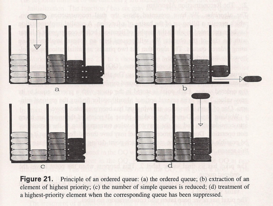
The reconstruction function corresponds to the "flooding" of a basin.
The relationship between the reconstruction and the Watershed Transform is as follows:
Given a minimum seed point, that is, the minimum grayscale value on some image, the watershed algorithm starts "flooding" the image. Intuitively, "flooding" is an operation of assigning a label to all the pixels that are adjacent to the seed point and have a higher grayscale value than the seed point.
Notice these two points here "adjacent" (to what? How to assess adjacency?) and "higher grayscale value" (Progressive "flooding" is essentially tracking the circumference of a basin at some height from its lowest point).
On the first step of this process, we start with a seed point. A seed point has 4 or 8 neighbours and in this case it would be very easy to decide which of those neighbouring pixels should be "flooded" in the next step.
But, as this process evolves, what started as a "seed point" now becomes a surface whose outer boundary can meander in any possible way. This "surface" is the surface of the flooded basin.
Mathematically, this is expressed on page 446 by:
$$W_{i+1}(f) = \left[IZ_{Z_{i+1}(f)}(X_i(f))\right] \cup m_{i+1}(f) $$
Where:
- $W$ is the surface of the watershed
- $IZ$ is the "Zone of Influence" of a section
- $Z$ is the lower section of the image $f$
- $f$ is the image itself (it is viewed here as a two dimensional function that maps a two dimensional set of integers to a grayscale value, that is $f : \mathbb{Z}^2 \rightarrow \mathbb{Z}$ or perhaps the more familiar $f(m,n)$ that would return the grayscale value of $f$ at point $m,n$).
- $X$ is the upper section of the image $f$
- $m$ is the set of local minima of $f$ at some level $i$.
The "Zone Of Influence" of a single point or more generally, of a region of points of interest is the set of points at a finite minimum geodesic distance from the region of interest. This is specified on page 438, in two steps, as:
$$z_X(Y_i) = \left\{ x \in X : \begin{matrix} d_X(x,Y_i) \text{ finite} \\ \forall j \neq i, d_X(x,Y_j) < d_X(x,Y_j) \end{matrix} \right\}$$
$$IZ_X(Y) = \bigcup_i z_X(Y_i)$$
Where:
- $z$ is the Zone of Influence
- $d$ is the geodesic distance between two points
- $x$ is a point in the region of interest
- $X$ is the region of interest
- $Y$ is the rest of the points in a specific image
BUT, as you can probably observe from the discussion so far all these quantities of interest are binary or come as the result of operations between binary objects. Remember that a grayscale image is some $f: \mathbb{Z}^2 \rightarrow \mathbb{Z}$, so, how do we calculate that $d$ which is then taking part in these "selection" operators?
Distances are calculated between sets of points (including point-to-point, expressed as a set of one element). A grayscale image contains numbers within the range defined by the pixel depth, how do we establish "distance" between any two of them?
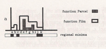
The "trick" (sic) to converting a grayscale image to a binary one is via the "sections". The sections are the first thing that is defined on page 434 as upper section $X_i(f) = \left\{ x \in \mathbb{Z}^2:f(x) \geq i \right\}$ and lower section $Z_i(f) = \left\{ x \in \mathbb{Z}^2:f(x) \leq i \right\}$.
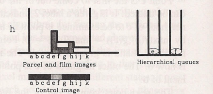
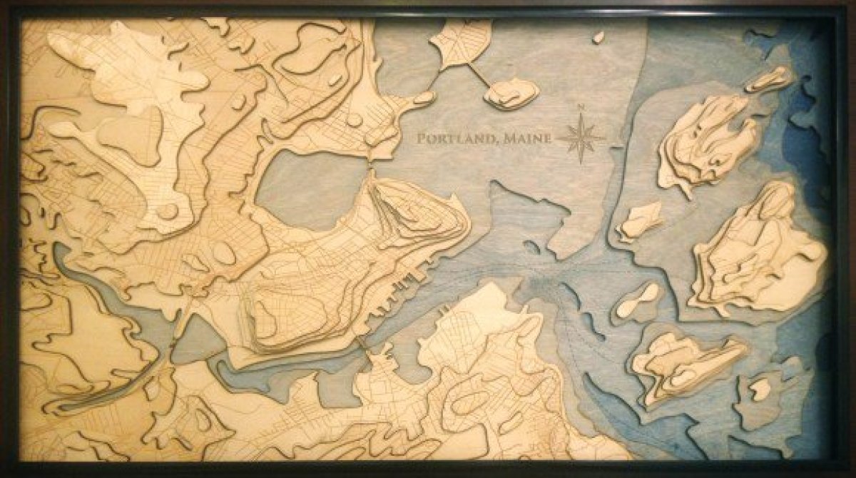
This is a view of an image as being composed of slices (sections) and looking roughly like this:

With this view in mind, it is now possible to compute geodesic distances between sections because they simply represent sets of points and therefore also possible to compute the reconstruction of a section. The reconstruction of a section refers to all the pixels that are at some finite distance from the section. This is the $R_X(Y) = \left\{ x \in X: \exists y \in Y, d_X(x,y) \text{finite} \right\}$ that is defined on page 437 and to a large part it drives the definition of the Zone Of Influence $IZ$.
The crucial point to note here is that if you derive $R$'s repetitively for each section $i$ of the image, these $R$'s will be "nested" and "tangential" to each other allowing them to be used to simulate this effect of "flooding" from lower levels to higher levels. This is explained on page 439 from "Consider two functions..." to "...The dual operation is a closing.".
In conclusion, given a grayscale image $f:\mathbb{Z}^2 \rightarrow \mathbb{Z}$, we define the upper and lower sections at grayscale level $i$ as $X_i$ and $Z_i$ respectively. Given a section and a metric of distance $d$, we define the reconstruction function $R$. The reconstruction function $R$ helps in defining the Zone of Influence $IZ$ which is what the Watershed Transform "tracks", over a number of iterations to perform the segmentation.
Hope this helps
(Image retrieved from google images)

