Even more on: Kalman filter for position and velocity

Question

As a follow-on to this great question...

I'm trying to implement the model in the referenced article (and referenced Wikipedia article), but I'm not getting the results I think I should be getting. Ultimate I would like to take this example and marry it with intermittent GPS data so as to simulate accelerometer failover in situations where GPS is lost.

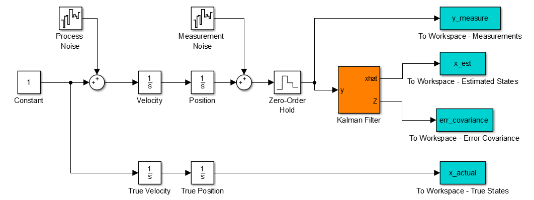
I've build the following model in Simulink:

UPDATED MODEL:

and power it using the following UPDATED Matlab code:

% Configure simulation
sim_length=10;
Ts=0.1;

% State space equations
A = [1 Ts;0 1];
C = [1 0];

% Noise characteristics
sigma_a = .1;
process_noise_power = 10;
measurement_noise_power = 10;

% Noise matrices
G = [(Ts^2)/2; Ts];
H = [1];

% Process noise
Q = sigma_a^2;
% Q = G*G'*sigma_a^2;

% Measurement noise
R = measurement_noise_power;

% Steps (not needed)
N = 0;

% Run simulation
sim('full_discrete_2inputs');

% Show results
close all;
figure(1);
hold on;
plot(tout,x_actual,'b-');
plot(tout(1:length(y_measure)),y_measure,'m-');
plot(tout(1:length(x_est)),x_est(:,1),'r-');
legend('True Position','Measured Position','Filtered Position','Location','Best');
title('Actual vs Kalman Filtered Position');
xlabel('Sample time [s]');
ylabel('Distance from origin [m]');
grid on;
hold off;
shg;

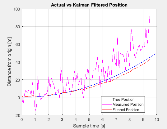
And here are my UPDATED results:

So with that, I have the following questions:

1. Did I inject the noise at the correct location? Is it appropriate to inject it prior to the double integration?
2. What's a good real-world noise power level to use in this application? I picked a number at random, but I imagine whatever I pick has to be considered in my Q or R matrices. I know if I bump the noise up to something like 50, the filter output and measurement value go wild, but still track each other.
3. To get the simulation to work I had to change my H matrix to 1, but [1 0] was specified in the example. Does anyone know why?

Answer 1

There are some problems:

1-Did I inject the noise at the correct location? Is it appropriate to inject it prior to the double integration?

The noise you injected accounts for process noise at the acceleration state, which you seem to assume as constant plus random disturbance. But then your true state generation is wrong.

2-What's a good real-world noise power level to use in this application? I picked a number at random, but I imagine whatever I pick has to be considered in my Q or R matrices. I know if I bump the noise up to something like 50, the filter output and measurement value go wild, but still track each other.

Which noise? Measurement or Process noise? Where is your measurement noise added? On the simulink model or on the script file?

3-To get the simulation to work I had to change my H matrix to 1, but [1 0] was specified in the example. Does anyone know why?

H =[1 0] is correct if your state $X = [x ~~\dot{x}]^T$ has 2 elements such as position $x$ and velocity $\dot{x}$. Becasue your measuring just the first state $x$, the position.