Lagrange parabolic estimator
The standard Lagrange polynomial parabolic interpolation peak finding formula from Peter's answer,
$$p = \frac{1}{2} \frac{\alpha - \gamma}{\alpha - 2\beta + \gamma}$$
has bias as function of the true delay $d$ if the cross-correlation peak is that of a critically sampled sinc. If the sampling frequency is increased, the sample values are increasingly dominated by the Taylor parabola of the cross-correlation centered at the peak, and Lagrange interpolation becomes more accurate. The Lagrange parabola adapts well to different peak shapes.
Lagrange parabolic estimator with bias correction
The bias as function of true delay $d$ in the peak time $p$ given by the Lagrange parabola can be corrected to zero bias by a post processing step:
$$d = \frac{\sqrt{32p^2 + 1} - 1}{8p}\tag{1}$$
There are no guarantees that the correction works for other peak shapes than critically sampled sinc.
Zero bias parabolic estimator
Here is presented a noise-robust estimator of the peak time that is zero-bias as function of $d$ if the cross-correlation is a noiseless delayed critically sampled sinc. Do not assume good performance if the sinc is not critically sampled or if you have another peak shape.
In the limit of zero white additive noise and with a uniform distribution of the fractional part of $d$ the new estimate has a root-mean-square error of about $0.84416936$ times the root-mean-square error in the samples of a unit amplitude sinc, according to an error propagation analysis using partial derivatives of the sample errors. This figure is better than that of any other estimator of same functional form (a weighted sum of three successive sample values divided by another weighted sum of those) that has zero bias as function of $d.$ The delay estimate is:
$$p = \frac{\gamma - \alpha}{\alpha + 2 \beta + \gamma},\tag{2}$$
where $[\alpha,\,\beta,\,\gamma]$ are the sample values just before, at, and just after the largest sample, respectively. The property of the estimator being zero bias as function of $d$ can be expressed as:
$$\begin{array}{c}-2 < d < 2\\
[\alpha, \beta, \gamma] = \left[\operatorname{sinc}(-d-1),\, \operatorname{sinc}(-d),\, \operatorname{sinc}(-d+1)\right]\quad\Rightarrow\quad p = d\end{array}\tag{3}$$
Amplitude scaling of the sinc doesn't affect the zero bias property. The estimator can still be interpreted as finding the zero of the derivative of a parabola such as:
$$\frac{1}{2}(α + 2β + γ)p^2 + (α - γ)p,\tag{4}$$
which is really no good for interpolation of the amplitude. There may be another parabola that has the same zero of the derivative but can be used for approximate amplitude interpolation.
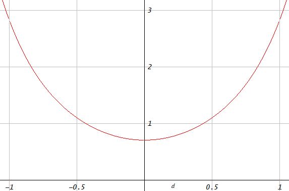
With a critically sampled delayed sinc as input, white noise sensitivity of the estimator depends on $d:$
$$\lim_{\operatorname{RMSE}_{[\alpha,\beta,\gamma]}\to0}\frac{\operatorname{RMSE}_{p}}{\operatorname{RMSE}_{[\alpha,\beta,\gamma]}} \approx \begin{cases}\frac{\sqrt{2}}{2}&\text{if }d=0,\\
2\sqrt{2}&\text{if }|d|=1,\\
\sqrt{\frac{\pi^2d^2(d + 1)^2(d - 1)^2(3d^2 + 1)}{2\sin^2(\pi d)}}&\text{otherwise},\end{cases}\tag{5}$$
where $\operatorname{RMSE}$ stands for root mean square error.

Figure 1. White noise sensitivity as function of $d$ (plot of Eq. 5).
Comparison
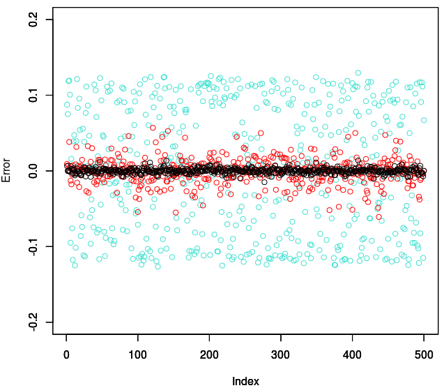
A variation of the R script in Peter's answer randomizes also delay lengths in addition to the test signal samples, and produces these errors in the delay estimate for the different estimators:

Figure 2. Errors in the delay time estimate for 500 simulation runs, with standard deviation in parenthesis. Turquoise: Lagrange parabola (0.08), red: zero bias parabolic estimator (0.016), black: Lagrange parabola with bias correction (0.004).
In this case the lagrange parabolic estimator with bias correction would be the best choice to take, because it gives the least severe errors.
The R script that created Fig. 2:
library(signal)

sinc <- function(omega)
{
  #Taylor approximation near omega=0
  return((abs(omega) < 10^-10)*(- (pi*omega)^6/5040 + (pi*omega)^4/120 - (pi*omega)^2/6 + 1) + (abs(omega) >= 10^-10)*sin(pi*omega)/(pi*omega) )
}

fractional_delay_filter <- function(delay, length)
{
  eps <- 10^-10
  t <- seq(0,length-1)
  t[t == 0 ] <- eps
  filter <- sinc(t-delay)
  return(filter)
}

# Lagrange parabolic
peak_location1  <- function(ykm1,yk,ykp1)
{
  return(0.5*(ykm1 - ykp1)/(ykm1 - 2*yk + ykp1))
}

# Robust zero-bias parabolic
peak_location2  <- function(ykm1,yk,ykp1)
{
  return((ykp1 - ykm1)/(ykm1 + 2*yk + ykp1))
}

# Lagrange parabolic with correction
peak_location3  <- function(ykm1,yk,ykp1)
{
  p <- 0.5*(ykm1 - ykp1)/(ykm1 - 2*yk + ykp1)
  return((sqrt(32*p^2 + 1) - 1)/(8*p))
}

estimate_delay <- function(x,xd,locator)
{
  cc <- ccf(xd,x,plot=F)
  idx <- which.max(cc$acf)
  return(locator(cc$acf[idx-1], cc$acf[idx], cc$acf[idx+1]) + cc$lag[idx])
}

Nres <- 500

true_delay_frac <- matrix(, nrow = Nres, ncol = 1)
errors <- matrix(, nrow = Nres, ncol = 3)
for (n in seq(1,Nres))
{
  true_delay <- runif(1, 10, 11)
  d5p1 <- fractional_delay_filter(true_delay,32)

  T <- 1000

  x <- rnorm(T,1)
  xd <- filter(d5p1, 1, x)

  true_delay_frac[n, 1] <- true_delay - 10;
  errors[n, 1] <- estimate_delay(x,xd[1:T],peak_location1)-true_delay
  errors[n, 2] <- estimate_delay(x,xd[1:T],peak_location2)-true_delay
  errors[n, 3] <- estimate_delay(x,xd[1:T],peak_location3)-true_delay
}

plot(errors[,1],col='turquoise', ylab="", ylim=c(-0.2,0.2))
par(new=T)
plot(errors[,2],col='red', ylab="", ylim=c(-0.2,0.2))
par(new=T)
plot(errors[,3],col='black', ylab="Error", ylim=c(-0.2,0.2), xlab="Index")
par(new=F)
title('Delay estimation error')

sqrt(var(errors[,1]))
sqrt(var(errors[,2]))
sqrt(var(errors[,3]))

