But why we use prediction filter?
To reduce the error we would have by encoding the actual sample directly.
How does the filter do that?
By combining past values in a clever way. If you are disturbed by filter, you can call it (linear) extrapolation, just a different way of looking at it.
DPCM may encode signals more efficiently, using the past known values.
For instance, dealing with a sampled signal (would work in a similar manner for analog signals), the idea is to encode:
- on a smaller size (less bits), with the same precision as the original signal (as a form of lossless compression),
- on a smaller size (less bits), with better precision than if one had quantized the original signal to that smaller size, sample per sample (as a form of lossy compression).
The hypothesis is that past values can predict, more or less faithfully, the actual value. This tends to work poorly for random data, but generally works fine, on average, for signals bearing information, that is, having some regularity.
For instance, if the signal looks (a least on a short time period) like a line, you can predict ${x}[0]$ from previous samples ${x} [-1]$ and ${x} [-2]$ with
$$\hat{x}[0] = 2{x}[-1]- {x}[-2]\,.$$
Do not forget that the older sampled (could) have been previously quantified: we write them ${x}_Q[-1]$ and ${x}_Q[-2]$, so actually:
$$\hat{x}[0] = 2{x}_Q[-1]- {x}_Q[-2]\,.$$
Even if your signal is not exactly linear, you can expect that, quite often, the prediction error $e[0]={x}[0]-\hat{x}[0]$ will be smaller than ${x}[0]$. Hence, if you quantize ${x}[0]-\hat{x}[0]$ instead of ${x}[0]$, with the quantization function $\mathcal{Q}$, you can reconstruct the final ${x}_Q[0]$ as:
$$\mathcal{Q}(e[0])+2{x}_Q[-1]- {x}_Q[-2]\,,$$
hopefully closer to $x[0]$ than with a direct quantization $\mathcal{Q}(x[0])$.
Of course, you can use more samples from the past, prediction functions different from a linear combination, pre-processing on the samples, adaptive modification of the coefficients (ADPCM).
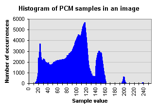
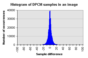
From An illustration of DPCM's advantages over PCM, you can see the interest, looking at histograms. Suppose you want to requantize an image, its histogram is:

and its DPCM histogram is:

As the second histogram contains all the necessary information to reconstruct the image, and is better concentrated around $0$ values, with very few high values, apply $\mathcal{Q}$ on it results in smaller errors than applying $\mathcal{Q}$ on the first histogram.


