I find the diagonal term a bit confusing. Sometimes, for wavelets, people separate scalar and vector or block thresholding. [EDIT] Now I believe I understand it. If you put all your samples or coefficients in a long 1D vector, then multiplying it by a diagonal matrix yield a scalar operation. With non-diagonal, you allow cross-terms.
For structured signals, or images, or transformed signals (in a wavelet or a time-frequency domain), neighboring samples or coefficients often possess some local correlations, that you want to exploit in denoising. So assume you have an observation $r(k)$ at location $k$ (could be multidimensional), and look for an estimator $\hat{s}(k)$ of some underlying signal $s(k)$, under a noisy model $r(k) = s(k)+n(k)$. In the original domain, you could for instance apply a scalar mask $f(k)$ on the observation: $\hat{s}(k) = f(k).r(k)$, especially if you know that at some location you have signal, at other noise. Windowing is a typical example. More generally, you can apply a function $f$: $\hat{s}(k) = f(r(k))$. If you assume local correlations, you can borrow information for close samples. For instance, average filtering can be $\hat{s}(k) = \frac{1}{3}(r(k-1)+r(k)+r(k+1))$.
In other words, $f$ now apply over a domain, gathered in a vector $v(k)= [r(k-1),r(k),r(k+1)]$. It can be called Reference Observation Vector (ROV). Then $\hat{s}(k) = f(v(k))$. So average filters are sort of non-diagonal processing.
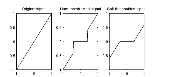
Traditionnaly with wavelets or time-frequency, the transform compacts or sparsifies noisy data, and data features tends to become relatively higher than the noise, compared to the original domain. So the previous idea of a scalar mask works better. You can choose $f$ to keep the value of $r(k)$ if $|r(k)|$ is above a threshold $t$, and set it to zero if below. This $f$ is discontinuous. let us write it $f(x) = \mathrm{sign}(x) (|x|-t)_+$
This is called scalar wavelet shrinkage or thresholding, scalar because you apply it on a single wavelet coefficient, illustrated in the center plot.

This idea was already used in the Fourier domain for noise reduction in speech. You can have smoother transistion, if you attenuate a bit the higher values, which give you soft thresholding, and you have many more shrinkage functions (garrote, firm) for scalar thresholding.
The next idea is to combine all of the above. You can modify one coefficient with respect to a certain norm of a surrounding $\|v(k)\|$, as:
$\hat{s}(k) = f(\|v(k)\|)r(k).$.
In wavelets, the ROV $v(k)$ can be more complicated. It can gather neighbors of the coefficients, but also coefficients from other scales.
The rationale is that, if a coefficient is small, it might be useful to preserve it anyway. If its ROV has high norm (think of energy), the coefficient might small by mistake, and is not noise.
The nice think is that the Stein Unbiased Risk Estimator theory allows you to estimate something on the signal $s(k)$ that you do not know by using only the observation $r(k)$, using some technical conditions, which allows you to find, automatically, the best threshold $t$, or shape paramaters of the function $f$. Such methods yielded almost the state-of-the-art on wavelet denoising. I am not familiar with audio. However, for multispectral images, here is an example:
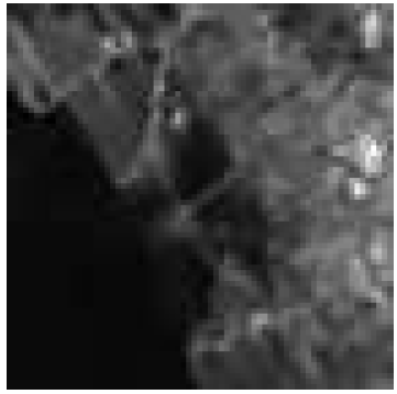
- a satellite image of the port of Tunis:

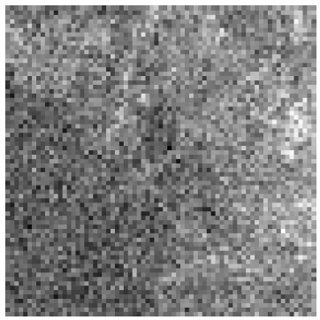
- its noisy version, with heavy Gaussian noise:


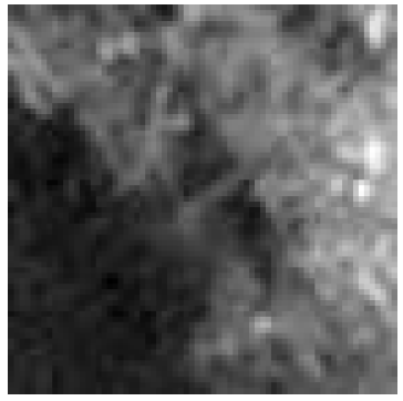
While not perfect, it was able to recover details, almost invisible from the noisy image, with very few parameters to set (only the shape of the ROV). This answer is a short version of what you can read in A Nonlinear Stein-Based Estimator for Multichannel Image Denoising, 2008.
Why can block denoising be better that scalar? Because scalar is a specific case of block (non-diagonal) processing, if you take the ROV to be restricted to the coefficient $r(k)$ itself. If you choose the time-frequency or time-scale method well, and the other parameters (block shape and size), the block processing is generally (much) better.

