Reconstruct FIR frequency response from the coefficients

Question

There is a lot of tools for designing FIR filters. Using one such tool I have designed a filter that satisfies my needs. It's coefficients are as follows:

 0.000106519966569472
 0.000164942422133671
 0.000154198611135164
-0.000051344150552581
-0.000527514219352601
-0.001228193882673074
 ...
 0.176493072494376790
 ...

In my system, 0.0001 / 0.1764 is about the same as ADC noise (well, not quite, but close). I'd like to know if a shorter filter, with some taps stripped off (zeroed) on either side still satisfies my requirements. This could be done by taking the modified array of the coefficients and reconstructing the frequency response of the modified filter.

Any tools for it (the cheaper the better)?

Edit

The tool works great. I post the result below. Good news is that only higher frequency response is visibly altered. Bad news is that by quite a lot. I am more interested in pass-band and slope, but I will look at more filter design tools to see if any of them has this sort of tradeoff built in. Thanks jojek.

Answer 1

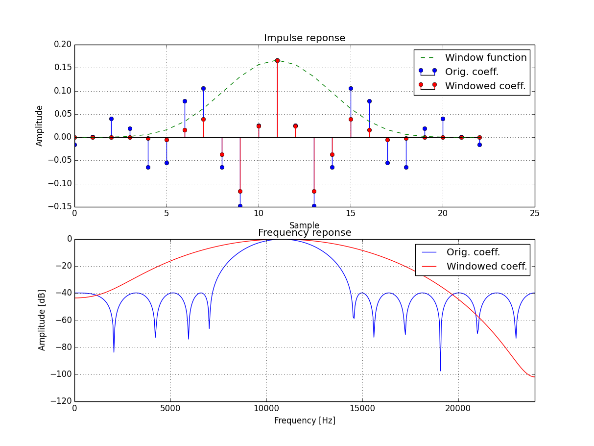
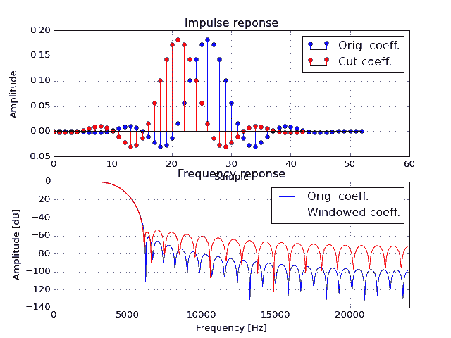
You can try to window the filter with some window function, i.e. Gaussian, to get rid of small coefficients (taper them). Although it won't really work very well and you might really want to think about redesigning your filter - it's the best solution in my opinion.

Here is an example for a bandpass filter, showing that it is not really working well and is affecting the frequency response. Everything is done in Python so presumably it's meeting your requirements of not spending a single penny.

Code is as follows:

import numpy as np
import matplotlib.pyplot as plt

# Some sampling frequency
fs = 48000.0    
# Size of FFT analysis
N = 1024

def fir_freqz(b):
    # Get the frequency response
    X = np.fft.fft(b, N)
    # Take the magnitude
    Xm = np.abs(X)
    # Convert the magnitude to decibel scale
    Xdb = 20*np.log10(Xm/Xm.max())
    # Frequency vector
    f = np.arange(N)*fs/N        

    return Xdb, f

if __name__ == "__main__":

    # FIR filter coefficients
    b = np.array([-0.0159147603287189,  0.000745724267485,  
                   0.0404251831063147,  0.019042013872129,  
                  -0.0644535904607569, -0.054523709591490,
                   0.0787623967281351,  0.105430811100048,
                  -0.0645610841865355, -0.148306808873938,
                   0.0257418551415616,  0.166568575042643,
                   0.0257418551415616, -0.148306808873938,
                  -0.0645610841865355,  0.105430811100048,
                   0.0787623967281351, -0.054523709591490,
                  -0.0644535904607569,  0.019042013872129,
                   0.0404251831063147,  0.000745724267485,
                  -0.0159147603287189])

    # Window to be used
    win = np.kaiser(len(b), 15)
    # Windowed filter coefficients
    b_win = win*b

    # Get frequency response of filter
    Xdb, f = fir_freqz(b)
    # ... and it mirrored version
    Xdb_win, f = fir_freqz(b_win)


    # Plot the impulse response
    plt.subplot(211)
    plt.stem(b, linefmt='b-', markerfmt='bo', basefmt='k-', label='Orig. coeff.')
    plt.grid(True)
    plt.hold(True)
    plt.stem(b_win, linefmt='r-', markerfmt='ro', basefmt='k-', label='Windowed coeff.')
    plt.plot(win*b.max(), '--g', label='Window function')

    plt.title('Impulse reponse')
    plt.xlabel('Sample')
    plt.ylabel('Amplitude')
    plt.legend()

    # Plot the frequency response
    plt.subplot(212)
    plt.plot(f, Xdb, 'b', label='Orig. coeff.')
    plt.grid(True)
    plt.hold(True)
    plt.plot(f, Xdb_win, 'r', label='Windowed coeff.')

    plt.title('Frequency reponse')
    plt.xlabel('Frequency [Hz]')
    plt.ylabel('Amplitude [dB]')
    plt.xlim((0, fs/2)) # Set the frequency limit - being lazy
    plt.legend()

    plt.show()

Answer 2

You could use a smooth window function to make the filter shorter, i.e. you multiply the coefficient vector element-wise by a shorter window function in a way that you only get rid of the small coefficients on both ends of the impulse response. Performing an FFT on the windowed filter coefficients will show you if the filter still satisfies your specs. BUT, why don't you just use the filter design tool to design another shorter filter and see if it satisfies the specs? This second approach will most likely yield a better filter for a given filter length than the first one.