Your filter is the all-poles IIR, this simplifies things a bit. Normally you can write transfer function in following form:
$H(z)=\dfrac{\sum_{i=0}^{P}b_{i}z^{-i}}{\sum_{j=0}^{Q}a_{j}z^{-j}} $
Going back to the discrete time domain you will get:
$y[n] =\dfrac{1}{a_0}\left( \sum_{i=0}^{P}b_ix[n-i]-\sum_{j=1}^{Q}a_jy[n-j]\right)$
Therefore in your case it is:
$y[n]=x[n]-0.1y[n-30]$
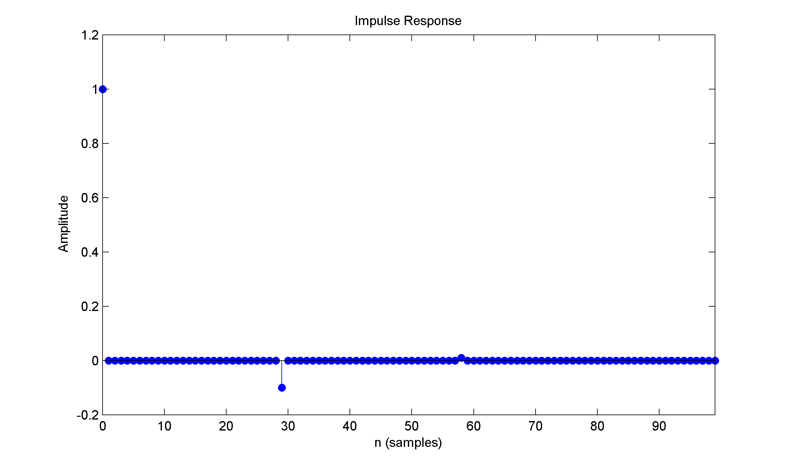
Calculation of particular values can be done by feeding Kronecker delta to your system ([1 0 0 0 0 0 0 ...] signal). Basically you will observe that something is happening every 30 samples ;) You can easily generate the plot in MATLAB/Octave, just remember that your filter has following coefficients:
b=[1]
a=[1 0 0 0 0 0 0 0 0 0 0 0 0 0 0 0 0 0 0 0 0 0 0 0 0 0 0 0 0 0.1]
By calling impz(b,a) function you will get similar plot (first 100 samples):


