defining the frequency range with fast fourier transform

Question

In the following example I have used various examples found on the web to understand fft and detecting signals with matlab.

fs = 1000; 
t = 0:1/fs:1.5-1/fs; 

x = 3*cos(2*pi*20*t + 0.2) + 1*cos(2*pi*30*t + 0.3) + 2*cos(2*pi*40*t + 2.4);
N = length(x);

% define the frequency components of the series 
freq = 0:N-1;
freq = freq*fs/N;

% normalise the data and compute the fourier transform
X = fft(x)./N; 
cutOff = ceil(N/2);
X = X(1:cutOff);
freq = freq(1:cutOff);

figure;
stem(freq,abs(X));
xlabel('frequency');
ylabel('amplitude');

Resulting in:

Why is it that the amplitude of the final plot are 1.5, 0.5, and 1 respectively? The initial amplitudes were 3, 1, and 2 so why is the amplitude of the signal half of that?

Also, could someone explain the section

% define the frequency components of the series 
freq = 0:N-1;
freq = freq*fs/N;

I don't quite understand how this works.

Answer 1

There are a few things going on here. First, one of the fundamental properties of the Fourier transform is that it conserves energy, i.e. the energy of the time domain is exactly equal to the energy of its Fourier transform. What is the power of a sinusoid? Assuming we restrict the calculation to integer multiples of cycles it is as follows (I suggest working out this equation for yourself if you are not sure about it):

$$ P(Asin(ft)) = \frac{A^2}{2} $$

The energy of a sinusoid is thus $\frac{A^2}{2}T$, or, in the case of discrete data, $\frac{A^2}{2}N$. The purpose of the following line of code-

X = fft(x)./N;

is to change the FFT output from an energy-based measure to a power-based measure ("based" because you have to square the transform results, just like you would in the time domain, to get the actual energy or power). Power is usually more interesting since it is an inherent characteristic of the signal, whereas energy is dependent on the number of samples that you are using.

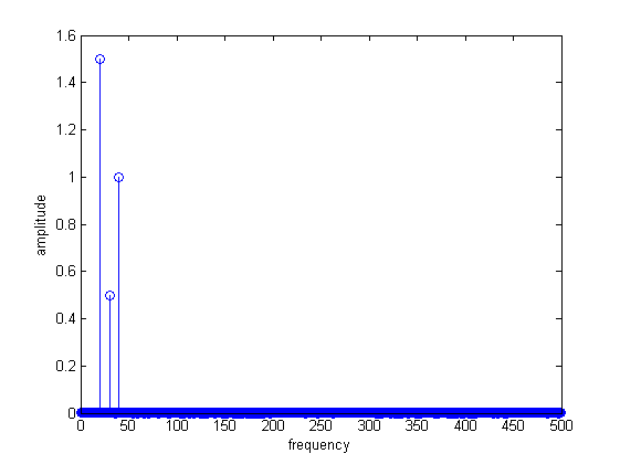
So, the power of your sinusoids is, according to the equation, 4.5, 2, and 0.5. You got 1.5, 1, and 0.5, which, if you square them, become 2.25, 1, and 0.25. You will notice that those results are exactly one half your expected power. The reason for the halving is that you are only showing the positive frequencies from your Fourier transform. That is what the following lines of code are doing-

cutOff = ceil(N/2);
X = X(1:cutOff);

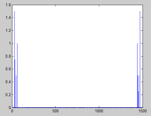
They are cutting off the negative frequency part of the spectrum. If you plotted the entire set of results it would look like the following-

The spikes on the left are the positive frequencies that you saw before. The spikes on the right are the negative frequency components of the sinusoids. Note that they have the exact same magnitude as their positive frequency partners, and thus comprise the missing factor of two in the power.

Lastly, you ask the following-

Also, could someone explain the section

% define the frequency components of the series 
freq = 0:N-1;
freq = freq*fs/N;

Samples sampled at frequency $f_s$ can represent frequencies from $-\frac{f_s}{2}$ to $\frac{f_s}{2}$ (see Nyquist Sampling Theorem), or, equivalently, frequencies from $0$ to $f_s$ (see aliasing). The code implicitly assumes that the samples represent from $0$ to $f_s$.