Trying to simulate a Fourier transform spectrometer in Python

Question

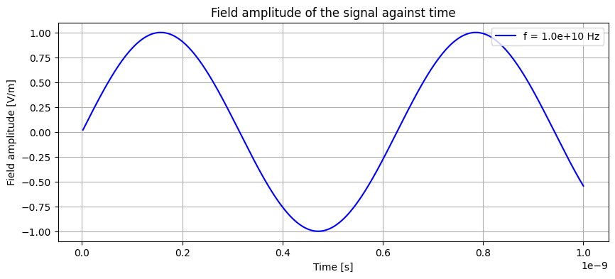
I'm trying to simulate a Fourier transform spectrometer in Python. I started basically with a simple single frequency (f=1e10 Hz) sine signal coming into the spectrometer. I obtained the following plot of the signal against time:

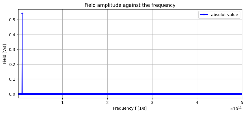
What the spectrometer is measuring is only the intensity of this signal - that is, the field amplitude squared. I plotted the field amplitude against frequency, so what I should obtain on my detector:

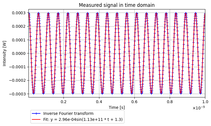
Now I did the inverse Fourier of my intensity and plotted the amplitude of my obtained signal against time:

As you can see, I fitted the signal that I obtained, and I don't get back the frequency that I settled at the beginning, so my code is not working. I don't understand why.

Here is my code (it's quite long I'm sorry but I'm stuck.):

import numpy as np
import matplotlib.pyplot as plt
import cmath
import scipy #for integral
from scipy.integrate import quad #for integral of kinf function f(x) between range a and b over x
from scipy import optimize
from scipy.fft import fft, fftfreq

# define constants
c = 3 * 10e8 # m/s, c = omega / k

#define variables
f = 10e9 #Hz
phi = 0 # phase à l'origine en rad (souvent fixée par l'expérimentateur)
# set the frequency range over which the integral will be calculated
f_min = 1e9
f_max = 500e9    

# number of sample
N = 1000
#sample maximal value
M = 8e-9 # in s
#samples spacing
S = M / N # 1/s 

# define time range
time_range = np.linspace(1/f_max, 1/f_min, N)

#create an array of the signal as a function of time
signal_in_time = 1 * np.sin(f * time_range + phi)

# plot of the signal of frequency w against time
plt.figure(figsize=(10,4))
plt.plot(time_range, signal_in_time, color = 'b', label ='f = {:.1e} Hz'.format(f))
plt.xlabel('Time [s]')
plt.ylabel('Field amplitude [V/m]')
plt.title('Field amplitude of the signal against time')
plt.legend(loc='upper right')
plt.grid()

   # store this signal in an array of signal measured at every frequency: there is only one signal at frequency w
field_amplitude = np.zeros(N)

    # define frequency range
    frequency_range = np.linspace(f_min, f_max, N)

# store this signal at the slice of the array of corresponding ferquency 
j=0
for i in frequency_range:
    #print('{:e}'.format(i))
    #print(i)
    if i == 9990990990.990992:
        print('BINGO')
        field_amplitude[j] = sin
        j += 1
    else:
        j += 1

#print(field_amplitude)

# in this cell, do the inverse Fourier transform of the Field versus angular frequency array

# array of intensity: here just square of amplitude array
intensity = field_amplitude * field_amplitude 

#inverse Fourier of the intensity
inv_four = np.fft.ifft(intensity)

# define the x axis for the plot of the signal
time_range = np.linspace(1/500e9, 1/1e9, N)    

# Plot of the Intensity (inverse Fourier transform of the incident power) versus time
plt.figure(figsize=(8,4))
plt.plot(time_range, inv_four.real, '+-', color = 'b', label = 'Inverse Fourier transform')
plt.xlabel('Time [s]')
plt.ylabel('Intensity [W]')
plt.title('Measured signal in time domain')
plt.ticklabel_format(useMathText=True)
plt.xlim(np.min(time_range), np.max(time_range))
plt.grid()
plt.legend(loc='center left', bbox_to_anchor=(0, -0.22))
plt.show()    


#define a sinus function to fit the measured signal
def sin_fit(x, a, b, c):
    return  a * np.sin(b * x + c)

# sin = 1 * np.sin(f * 1e-9 + phi)

# do the fit
params, params_covariance = optimize.curve_fit(sin_fit, time_range, inv_four.real, p0=[0.0003, 11.3e+10, +0.9])

a = params[0]
b = params[1]
c = params[2]
print('the parameters found by the fits are: ', params)


print('Angular frequency of the signal that is set:  {:2e}'.format(f))
print('Angular frequency found by Fourier transform: {:2e}'.format(b))

# Plot of the Intensity (inverse Fourier transform of the incident power) versus time
plt.figure(figsize=(8,4))
plt.plot(time_range, inv_four.real, '+-', color = 'b', label = 'Inverse Fourier transform')
plt.plot(time_range, sin_fit(time_range, a, b, c), '-', color = 'r', label = 'Fit: y = {:.2e}'.format(a) +'sin({:.2e} * t'.format(b) + ' + {:.2})'.format(c))
#plt.plot(time_range, sin_fit(time_range, 0.0003,11.3e+10, +0.9), color = 'orange')
plt.xlabel('Time [s]')
plt.ylabel('Intensity [W]')
plt.title('Measured signal in time domain')
plt.ticklabel_format(useMathText=True)
plt.xlim(np.min(time_range), np.max(time_range))
plt.grid()
plt.legend(loc='center left', bbox_to_anchor=(0, -0.22))
plt.show()

Answer 1

The OP is trying to recover the time domain signal by taking the inverse FFT of the "intensity", I assume because that would be the only information available in an actual test (so amplitude vs frequency from the power spectrum, and no phase).

The inverse FFT will result in a matching sinusoid (with arbitrary phase offset since the phase is not known). I believe the reason for the mismatch is because the OP did not use a frequency axis representing the FFT corresponding to the sampling frequency used (along with slight error in the way the time was indexed).

An FFT with $N$ samples with a frequency index typically as $k$ with $k$ going from $k=0$ up to $k=N-1$, corresponds to a frequency axis that starts with "DC" (which means direct current from EE terminology as a short hand for 0 frequency like a DC battery), and extends to nearly the sampling rate ($k=N$ corresponds to the sampling rate exactly).

If we review the OP's data, the sampling rate can be derived from the time axis that was created (subtract one sample from the previous to get $\Delta T$ and $f_s = 1/\Delta T$. I did this and got a sampling rate of 1.001002 THz (nearly 1E12). We then see from the plot the OP provided showing the amplitudes for each frequency that it only goes to 5E11: So the OP used a frequency axis of DC to half the sampling rate instead of what I defined above. From the code we see the OP intended to model a sinusoid at 10 GHz but instead got something nearly twice this (18 GHz) consistent with the frequency axis being half as long with the additional errors in the time indexing used, and visually from the OP's plot, we see 18 cycles in 1E-9 seconds: 18 GHz.

So to properly do what the OP is intending, the following can be done:

Create a frequency domain waveform with $N$ samples (starting with all zeros for now, we will fill the proper frequency bins in a subsequent step) where $N$ corresponds to sampling rate and time duration of the capture according to:

$$N = f_s T$$

Where:

$f_s$ is the sampling rate in Hz
$N$ is the total number of samples (in time AND in frequency)
$T$ is the total time duration in seconds

For example if we want to simulate a 10 GHz tone and use an integer number of samples then we could use a 1 THz sampling rate (closest to the OP's case), and a total time duration of 1 cycle of the tone which is 1/10E9 = 1E-10 seconds (100 ps), OR 2 cycles of the tone which is 2E-10 seconds or any higher integer. This will result in exactly the case the OP has shown where all other FFT bins are zero. (We can use any other time durations, but then we have to pull spectral leakage into the discussion, and given the OP is less familiar with all that, I prefer to avoid that for getting initial results).

The next thing to know is the bin spacing, $f_\Delta$, which in Hz would be the sampling rate divided by the total number of samples:

$$f_\Delta = f_s/N$$

Note that this also corresponds directly to

$$f_\Delta = 1/T$$

A real sinusoid (perfectly sampled so that the frequency is directly on bin center) would have two non-real bins, one at index $k$ and the other at index $N-k$. (Just take the FFT of the test sine wave and plot the magnitude of the results to confirm this). If the sine wave used doesn't complete an exact integer number of cycles in the complete waveform used, additional spectral leakage will result but if we have an exact number of cycles in time, there will be only two non-real bins in frequency (I provide more details why at the very end).

So the final step now is to populate the proper bins for the frequency the OP desires. If the time duration chosen was $T= 1E-10$, then the first bin will correspond to the desired frequency of 10 GHz: The bin spacing is as $1/T$ in this case is 10 GHz, so if we count along the frequency axis in increments of $k$, we get $k=0 \rightarrow f=0$, $k=1 \rightarrow f=10$ GHz, $k=2 \rightarrow f=20$ GHz etc. So in this case we populate $k=1$ with a non-zero value, and as explained above, we also populate $N-k$ = $N-1$ with a non-zero value. Doing this will result in the correct sinusoidal frequency after processing the resulting array with the inverse FFT. If the time duration is doubled, then we would do this all with $k=2$ and $k=N-2$ instead, with all other bins zero.

Finally the time indexing can be done accurately using:

time = np.arange(N)*1/fs

In summary the solution is to properly extend the FFT samples all the way to one sample less than the corresponding sample rate ($N$ samples with $k=0$ to $N-1$ where $N$ is the sampling rate).

Why two bins?

The reason two bins are populated is because the Fourier Transform of a sinusoid (which the DFT is representing) corresponds to the coefficients of frequencies given as $e^{j\omega t}$ NOT $\cos(\omega t)$. The general expression $Ke^{j\phi}$ means a phasor that has magnitude $K$ and phase $\phi$, thus $e^{j\omega t}$ is a "spinning phasor" on a complex plane. The two are related using Euler's formula:

$$2\cos(\omega t) = e^{j\omega t} + e^{-j\omega t}$$

And thus a real sinusoid (either cosine or sine) would have two components in the Fourier Transform: one at a "positive frequency" (meaning the phasor spins clockwise) and one at a "negative frequency" a phasor of the same magnitude and conjugate phase so spinning counterclockwise. When two phasors are added on the complex plane, you can do this graphically by placing one at the end of the other, and thus the sum will always stay on the real axis. In short every real waveform must have for each positive frequency component a negative frequency component that is equal in magnitude and opposite in phase (which keeps the sum on the real axis). In the FFT, every sample in the upper half of the FFT (which the OP didn't include) represents all these negative frequencies.

Note I tried to keep it simple in the outlined procedure, but it is worth mentioning that even if one bin was populated, the resulting time domain waveform would just be $e^{j\omega t}$ instead of $\cos(\omega t)$ or $\sin(\omega t)$. But using the following relationship also from Euler (rearranging the sine and cosine to exponential conversions):

$$e^{j\omega t} = \cos(\omega t) + j\sin(\omega t) $$

So from the complex time domain result $e^{j\omega t}$ we can extract the waveform $\cos(\omega t)$ or $\sin(\omega t)$ just by taking the real or imaginary component. The primary issue here was that the OP did not extend the frequency axis used to correspond with the sampling rate (it was only extended to half the sampling rate), and did not accurately represent the time increments (that second part resulted in less error). Whether one bin or two bins get populated, we can still extract the resulting sinusoid.

Answer 2

What your code does has nothing to do with a Fourier-transform spectroscopy (spectrometry), as defined, for example, in the Fourier Transform spectroscopy Wiki article and the ThermoFisher Scientific's brochure Introduction to Fourier Transform Infrared Spectrometry.

While not being aware of your true intentions as concerning your writing this question, I'm taking for granted that you are going to simulate the working principle of a generic FT spectrometry instrument.

Look how the cited references define the Fourier Transform spectroscopy (FTS) working principle.

The Wiki article contrasts FTS instruments with monochromator-based instruments:

[In contrast to monochromator-based instruments], [r]ather than allowing only one wavelength at a time to pass through to the detector, this technique lets through a beam containing many different wavelengths of light at once, and measures the total beam intensity. Next, the beam is modified to contain a different combination of wavelengths, giving a second data point. This process is repeated many times. Afterwards, a computer takes all this data and works backwards to infer how much light there is at each wavelength.

The ThermoFisher Scientific's brochure elaborates on this in details (Section Why FT-IR?, page 4 of 8):

Most interferometers employ a beamsplitter which takes the incoming infrared beam and divides it into two optical beams. One beam reflects off of a flat mirror which is fixed in place. The other beam reflects off of a flat mirror which is on a mechanism which allows this mirror to move a very short distance (typically a few millimeters) away from the beamsplitter. The two beams reflect off of their respective mirrors and are recombined when they meet back at the beamsplitter. Because the path that one beam travels is a fixed length and the other is constantly changing as its mirror moves, the signal which exits the interferometer is the result of these two beams “interfering” with each other. The resulting signal is called an interferogram which has the unique property that every data point (a function of the moving mirror position) which makes up the signal has information about every infrared frequency which comes from the source.

This means that as the interferogram is measured, all frequencies are being measured simultaneously. Thus, the use of the interferometer results in extremely fast measurements.

Because the analyst requires a frequency spectrum (a plot of the intensity at each individual frequency) in order to make an identification, the measured interferogram signal can not be interpreted directly. A means of “decoding” the individual frequencies is required. This can be accomplished via a well-known mathematical technique called the Fourier transformation.

Unlike the steps described in both references leading to extraction of a frequency spectrum (a plot of the intensity at each individual frequency), presumably required by the analyst, your code performs only a Fourier transform of "the intensity at each individual frequency" and nothing else but fitting and plotting curves.

#...

# in this cell, do the inverse Fourier transform of the Field versus angular frequency array

# array of intensity: here just square of amplitude array
intensity = field_amplitude * field_amplitude 

#inverse Fourier of the intensity
inv_four = np.fft.ifft(intensity)

#...
# do the fit, print # Plot of the Intensity (inverse Fourier transform of the incident power) versus time

#...

In your code, you've got outright what the Fourier Transform spectroscopy aims to achieve (the intensity spectrum), so why do you bother to perform calculations? And, while there might exist applications where light intensity Fourier transform could be useful, the FTS is not one of those. Notice also that as the light intensity is a squared EM wave amplitude, and the Fourier transform is a linear operation, the interpretation of the Fourier transform of light intensity in terms of EM wave variables is not that straightforward, if ever possible without complicated processing.

At first, I've written only the last paragraph as a comment, but your question would attract visitors through web searches, and I've added references and discussion. Still, please do not rate this text as an answer, it is just an extended comment.