2D Frequency Domain Convolution Using FFT (Convolution Theorem)

Question

In the time domain I have an image matrix ($256x256$) and a gaussian blur kernel ($5x5$). I've used FFT within Matlab to convert both the image and kernel to the frequency domain as zero padded $260x260$ matrices ($N + M -1 = 256 + 5 -1 = 260$)

I then multiply the image matrix by the kernel and use IFFT to convert the result back to the time domain. When I try to display the result, it is just junk and doesn't resemble the original image with a gaussian blur like it should.

Here is the Matlab code I am using, where image = $256x256$ and kernel = $5x5$:

imagefreqdomain = fft2(image,260,260)

kernfreqdomain = fft2(kernel,260,260)

filtimagefreqdomain = imagefreqdomain * kernfreqdomain

filtimage = ifft2(filtimagefreqdomain)

What am I doing wrong? Thanks

Answer 1

Similar to your question Applying 2D Image Convolution in Frequency Domain with Replicate Border Conditions in MATLAB the issue is what happens when you multiply in 2D in frequency domain.

So few remarks about that:

1. Multiplying in frequency domain for discrete signals with finite support is equivalent to applying convolution in spatial domain under the assumption of cyclic / periodic boundary conditions.
2. In image processing we usually define per kernel the anchor pixel of the kernel. Usually it is marked as (0, 0) of the kernel. We also mostly set it as the center pixel (In Image Processing most kernels have odd length). When we pad the kernel to the size of the image we usually add zeros on its bottom and right. Which means its (0, 0) isn't aligned with the image.

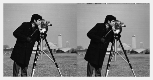
The misalignment with the circular boundary extension yields the following for the naïve code:

clear();
close('all');

gaussianKernelStd       = 0.5;
gaussianKernelRadius    = ceil(5 * gaussianKernelStd);

mI = im2double(imread('cameraman.tif'));
mI = mI(:, :, 1);

numRows = size(mI, 1);
numCols = size(mI, 2);

vX = [-gaussianKernelRadius:gaussianKernelRadius].';
vK = exp(-(vX .* vX) ./ (2 * gaussianKernelStd * gaussianKernelStd));
mK = vK * vK.';
mK = mK ./ sum(mK(:)); %<! The Gaussian Kernel


mIFiltered = ifft2(fft2(mI) .* fft2(mK, numRows, numCols), 'symmetric');
figure();
imshow([mI, mIFiltered]);

As you can see at the top and left filtered image (The right) has artifacts which are the result of the circular extension and the misalignment. How to fix it?
Well, padding the image correctly and padding with circular extension the kernel.
I showed it in Applying 2D Image Convolution in Frequency Domain with Replicate Border Conditions in MATLAB.