I'll illustrate with an example: detecting a rectangular pulse in noise, in Matlab.
Let's start with defining the signal that contains the pulse.
fs = 1/1000;
t = 0:fs:1;
s = [zeros(1,400), ones(1,100), zeros(1,501)];
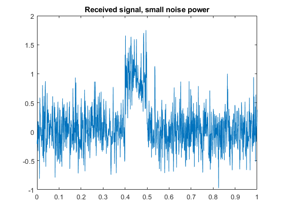
First let's do detection in noise with small power. We calculate the received (noisy) signal:
np = 0.1;  % noise power (variance)
n = sqrt(np)*randn(1,1001); % noise signal
r = s + n; % received signal
plot(t,r); title('Received signal, small noise power');

Now let's run the correlation:
c = xcorr(r,s);
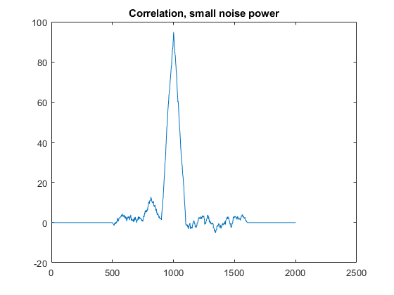
plot(c); title('Correlation, small noise power');

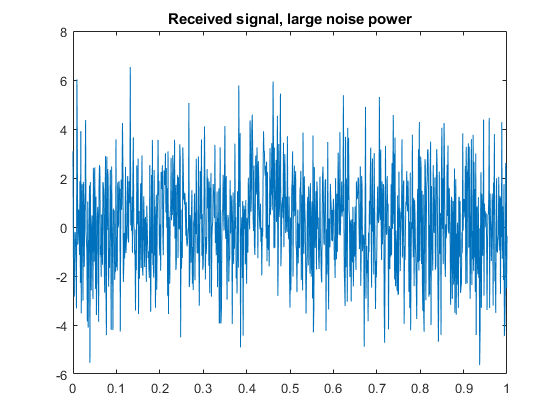
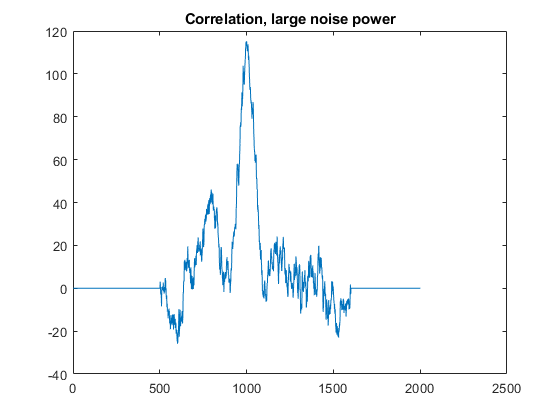
You can see how the correlation produced a large output, indicating that the pulse was there. What is amazing is that the correlator can find the pulse even when it is impossible for one to see it. Let us increase the noise power and repeat the process.
np = 4;
n = sqrt(np)*randn(1,1001);
r1 = s + n;  % received signal with large noise


As you can see, the correlator has an incredible ability to detect signals that are embedded in strong noise.
One thing you can do for yourself is run the correlation when the pulse is not present. The signal will be hard to distinguish from the noisy pulse shown above, but you'll see that the correlation does not produce a sharp maximum.
So, the implementation is quite easy; what is not so easy to do is:
- Prove that this technique produces the best possible signal to noise ratio at the correlation's peak.
- Determine the optimum threshold given some desired constraints on the probability of wrong detection (false positive or false negative).

