I have delved deeper into computer vision since first asking that question, and I have a better handle on real-world use-cases of DoG vs LoG. All of this signal processing basically boils down to looking for specific features, when you do not know a priori the scale that feature exists at. First, let us look at SIFT, Scale-invariant feature transform, specifically scale-space extrema detection.
SIFT
The scale space of a n-dim signal $f(x_0,x_1,\dots,x_n)$ is the family of derived signals $L(x_0,x_1,\dots,x_n; t)$, where $t$ is a tunable parameter corresponding to the scale of the filter, $t = \sigma^2$, or the variance of the Gaussian filter. To be more concrete, let us take a digital image $f(x, y)$ and create a 3D array $f(x, y, t)$ of $n_x \times n_y$ pixels and $n_t$ "slices", where each slice is a blurred copy of the original image for $t=\{0\dots n_t\}$, the first being 0 blurring, a.k.a. original image. Now for SIFT (simplification), apply an edge/corner detection to each slice, and correlate each point $corner(x,y)$ through $t$. When you have a strong number of these points detected, you can be confident that this is a keypoint of the image.
If you take the difference of any two different slices of $f(x,y,t)$, you get a DoG for $t_1$ and $t_2$.
Check out this page to see some examples of scale-space representation
SURF
SURF, or Speeded-up Robust Features, is an improvement on SIFT. This is a fantastic paper, and it, along with some of the papers it cites in Related Work, go much of the way to answer your question of "Have anyone looked into this further?"
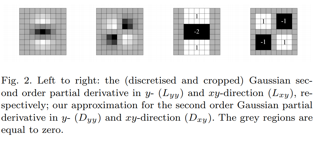
Here we get into the heart of the matter, why one might use LoG/DoG/Wavelet for a particular problem. Take a look at fig 2 on page 3:

These kernels approximate second-order Gaussian derivatives, which are objects normally of infinite width and resolution. However, because we are dealing with digital images, and also want to be fast, they are cropped, quantized, and discretized. However, once again, there are many choices for how we choose to crop and quantize, with pros and cons for each.
Wavelets

Wavelets are yet another approach to scaling, edge detection, etc. Wavelets have some nice mathematical properties which are beyond this scope. The picture above shows successive stages of discrete wavelet transform (DWT). The simplest wavelet is the Haar wavelet, $[1,-1]$, which is essentially the 1D discrete derivative, very similar to numpy.diff(array, axis=n). You apply your wavelet in one axis, which gives you a detail image $d_0$ (the edges) and an average image $a_0$. $a$ and $d$ are basically low-pass and high-pass outputs, respectively. In contrast to continuous filters, each time you apply a DWT, you get 2 outputs, each with half the number of pixels along the given axis. With 2d images, you will typically take a $m \times n$ image, apply a DWT in the vertical and in the horizontal, to get 4 images, $(d,d)$, $(d,a)$, $(a,d)$, and $(a,a)$. Your $(a,a)$ is the low-pass output in both directions, at half the resolution. You can apply DWT again, and again, recursively, each time getting an "octave" in scale space.
One obvious advantage of DWT is that each low-pass output has $\frac{1}{4}$ the number of pixels to process. The downside is you are limited to only octaves of scale space.
Continuous wavelet transform behaves in much the same way as Gaussian scale-space, except you specify not only the scale, but the filter kernel as well. In discrete images, different wavelets have different properties. The Daubechies wavelet is quite popular, because, insofar as I can tell, it works on magic.
deep breath Ok bear with me, almost done here.
Deep Convolutional Neural Networks

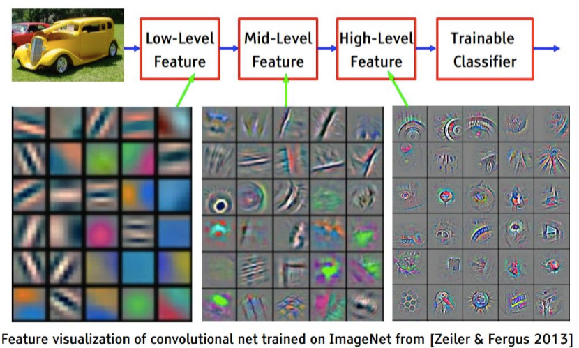
Feature-detecting filters in scale space show up in deep learning, but in this case, the convolutional kernels are learned, rather than specified by the scientist. Now, instead of tuning just $\sigma_1$ and $\sigma_2$, you have the entire network worth of architectures, parameters, and hyperparameters to fiddle with. Also your results are dependent on your image dataset. Your bandpass properties are completely beholden to your NN. But I think it's really cool that the NN is learning this of its own accord. No one said "let's have a neural network for images which uses successive edge detection for feature detection", they just created the convolutional neural network architecture, trained it on image classification tasks, and those filters just emerged as optimal solutions to the task.
Which is best? Of course, there is no single best for a given application. But here are some pros and cons:
- LoG: Simple, but has to be calculated for each scale. The discrete * LoG is a good approximation of the continuous. Basically a single parameter to tune.
- DoG: similar to LoG, but when generating a scale space, there is a lot of computational redundancy that can be leveraged to save time. Two parameters to tune, or more precisely, you chose window widths in scale space.
- DWT: Crazy fast, sometimes faster even than FFT. Limited to octave scaling. Choice of many discrete wavelets.
- CWT: similar to LoG, but with more choices of kernels, thus more knobs to twiddle.
- CNN: Great for real world datasets, but no direct over control tuning. Requires intensive training.
There is also a connection to Bessel functions to all this, if you want yet another rabbit hole.
(I've edited this answer and written it in several stages since there is a lot of content)


