Bandpass filters with python for low frequencies

Question

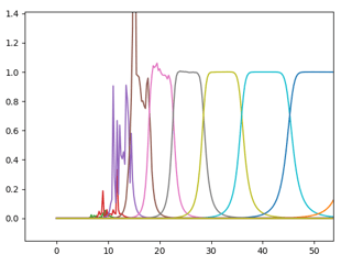
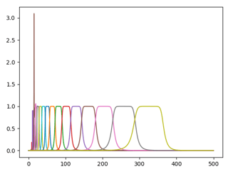
I have a signal, sampled at 1 kHz, that I would like to analyze in third octave bands. For that purpose I defined Butterworth filters with proportional bandwidth. This works well for higher frequencies, but produces very weird results for low frequencies. What am I missing? Plotted are the frequency responses of the Butterworth filters. I find similar behaviour in Hanning filters, and think that I am missing something fundamental.

Code used to define filters:

import scipy
import numpy as np
from scipy import signal
from matplotlib import pyplot as plt
def butter_bandpass(lowcut, highcut, fs, order=5, label=None):
    nyq = 0.5 * fs
    low = lowcut / nyq
    high = highcut / nyq
    b, a = signal.butter(order, [low, high], btype='band')
    w, h = signal.freqz(b,a,worN=2000)
    plt.plot((fs * 0.5 / np.pi) * w, abs(h), label=label)
    return b, a

center_freqs = np.array([0.5* 2 ** (n * 1 / 3.) for n in range(0, 29)])
center_freqs.sort()
lower_freqs = 2. ** (-1 / 6.) * center_freqs
for lf in lower_freqs:
    butter_bandpass(lf, lf*2**(1/3.), fs=1000, order=5)

plt.show()

Answer 1

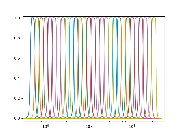
I would bet this is just numerical error in the transfer function. Try using butter_sos = butter(..., output='sos') instead of ba format, and sosfreqz(butter_sos, ...) instead of freqz. Does that fix it?

https://docs.scipy.org/doc/scipy-0.19.0/reference/generated/scipy.signal.sosfreqz.html

Edit: I just tried it and it does. :D

import scipy
import numpy as np
from scipy import signal
from matplotlib import pyplot as plt
def butter_bandpass(lowcut, highcut, fs, order=5, label=None):
    nyq = 0.5 * fs
    low = lowcut / nyq
    high = highcut / nyq
    sos = signal.butter(order, [low, high], btype='band', output='sos')
    w, h = signal.sosfreqz(sos,worN=20000)
    plt.semilogx((fs * 0.5 / np.pi) * w, abs(h), label=label)
    return sos

center_freqs = np.array([0.5* 2 ** (n * 1 / 3.) for n in range(0, 29)])
center_freqs.sort()
lower_freqs = 2. ** (-1 / 6.) * center_freqs
for lf in lower_freqs:
    butter_bandpass(lf, lf*2**(1/3.), fs=1000, order=5)

plt.show()

Answer 2

In general, IIR filters with transition bands that are a tiny fraction of the sample rate tend to become unstable (depending on the numerics used), due to the poles getting very close to the unit circle, and thus the state variables in the difference equations needing to accumulate both large enough numbers for the magnitude response, and really tiny fractions in order for the impulse response to last over a huge number of sample times, due to the low frequency cut-off relative to the sample rate.