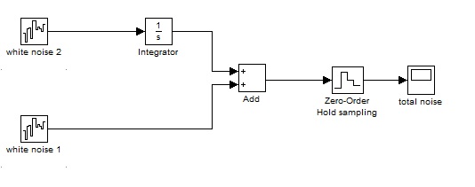
If the white noise has a Gaussian probability distribution, then it should be possible to find the variance of both noise sources using a power spectral density estimate.
$S_{1}(j\omega) = {\sigma_{1}}^{2}$ and $S_{2}(j\omega) = \frac{{\sigma_{2}}^{2}}{\omega^{2}}$, hence you should be able to minimize
$$
J(\sigma_{1},\sigma_{2}) = \| S_{1}(j\omega) + S_{2}(j\omega) - \hat{S}(j\omega) \|
$$
where $\hat{S}(j\omega)$ is the PSD estimate of your output, in order to find $\hat{\sigma}_{1},\hat{\sigma}_{2}$.
The MATLAB script below shows how this might work in practice.
Ts = 0.1; % sampling time
Nts = 1e6; % number of samples
n = randn(2,Nts); % two Gaussian noise sequences
t = (0:length(n)-1)*Ts; % time vector

sd = 1e3.*rand(1,2); % random standard deviations for noise signals

% filter for the noise
G = sd.*[tf(1,[1 0]), tf(1)];
% zero-order hold
Gd = c2d(G,Ts,'zoh');
% time-response for G(s) by the two Gaussian white noise sources
y = lsim(Gd,n,t);
y = y(1e2:end); % remove initial transient (only want stationary response)

% compute a PSD (of stationary response)
[Pxx,f] = pwelch(y,blackmanharris(length(y)/100),[],[],1/Ts,'psd','onesided');

% scaling using logarithm provides better numerical stability when
% minimizing the function
Jfun = @(p)(log(p(1)*1./(2*pi*f(2:end)).^2 + p(2)) - log(Pxx(2:end)));

p0 = 1e3.*rand(1,2); % random initial values for curve fit
p = lsqnonlin(Jfun,p0); % minimize the cost-function Jfun

sdh = sqrt(p/(2*Ts)); % estimate of standard deviations
est_error = norm(sd - sdh);

disp('Ideal parameters')
disp(sd)
disp('Estimated parameters')
disp(sdh)
disp('Estimation error')
disp(est_error)

fa = 10*log10(p(1)*1./(2*pi*f(2:end)).^2 + p(2));
figure(2), semilogx(f,10*log10(Pxx),f(2:end),fa), grid on
xlabel('Frequency'), ylabel('Power'), legend('PSD','Fit')

