Transfer functions for Scipy and Matlab's Butterworth filter don't seem to match theory

Question

The squared transfer function for a Butterworth filter of order $n$ should be

$$ |H(f)|^2 = \frac{1}{1+\left(\frac{f}{f_c}\right)^{2n}} $$

where $f_c$ is the cut-off frequency. (Here's one of many possible references.)

I'm unable to correctly reproduce this with either Python or Matlab. For example, let's say I want a third-order filter ($n=3$) with a $f_\mathrm{c}$ = 20 Hz cut-off frequency for a signal sampled at $f_\mathrm{s}$ = 100 Hz.

In Python, I would implement this as

import numpy as np
import matplotlib.pyplot as plt
from scipy.signal import butter, sosfreqz

fc = 20  # Hz, Cut-off frequency
fs = 100  # Hz, sampling frequency
order = 3  # Filter order

nyq = 0.5*fs  # Nyquist frequency
sos = butter(order, fc/nyq, analog=False, btype='low', output='sos')

w, h = sosfreqz(sos, worN=2000)
f = nyq*w/np.pi  # Convert to Hz

Hf2_scipy = np.abs(h)**2
Hf2_theory = 1/(1+(f/fc)**(2*order))

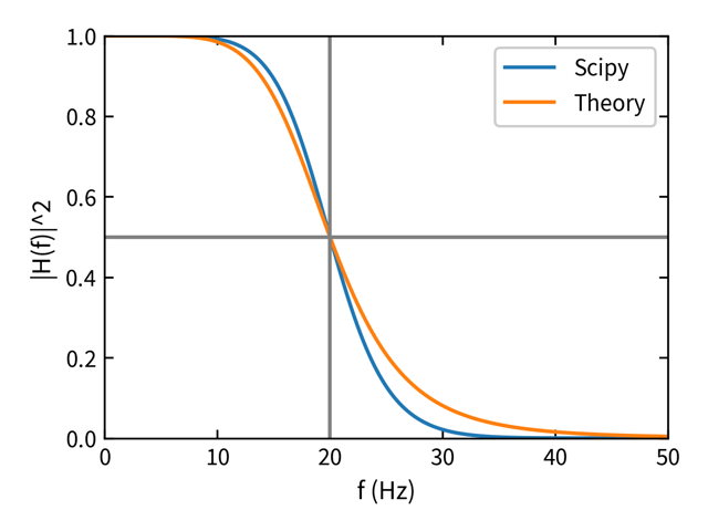
Plotting the result gives curves that don't match

fig, ax = plt.subplots()
ax.plot(f, Hf2_scipy, label='Scipy')
ax.plot(f, Hf2_theory, label='Theory')
ax.set(xlabel='f (Hz)', ylabel='|H(f)|^2', xlim=[0, nyq], ylim=[0, 1])
ax.axhline(0.5, color='0.5')
ax.axvline(fc, color='0.5')
ax.legend()

What am I missing?

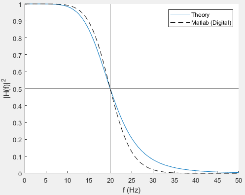
Here's the equivalent attempt in Matlab, which produces the same result

fc = 20;  % Cut-off frequency
fs = 100;  % Sample frequency
order = 3;  % Filter order

[z, p, k] = butter(order, fc/(fs/2), 'low');
sos = zp2sos(z, p, k);
[h, w] = freqz(sos, 2000);
f = w*fs/(2*pi); % Convert to Hz

Hf2_matlab = abs(h).^2;
Hf2_theory = 1./(1+(f/fc).^(2*order));
plot(f, Hf2_matlab, 'k')
plot(f, Hf2_theory)

plot([fc, fc], [0, 1], 'color', 0.5*[1, 1, 1])
plot([0, fs/2], [0.5, 0.5], 'color', 0.5*[1, 1, 1])
legend('Matlab', 'Theory')
xlabel('f (Hz)')
ylabel('|H(f)|^2')

Answer 1

It has to do with the Bilinear Transform, as Hilmar already stated.

The theoretical function is defined for the analog domain, so inherently there will be differences when you convert the response to the digital domain. However, you can still generate the "analog" frequency response and yield the expected result.

I took your code and added/modified it a bit to produce two plots: each comparing theory against the digital or analog version of the filter. This is done in MATLAB:

And here's the code:

%% Butterworth filter definitions

fc = 20;  % Cut-off frequency
fs = 100;  % Sample frequency
order = 3;  % Filter order

% Zero-pole gain definition for digital Butterworth filter
[z, p, k] = butter(order, fc/(fs/2), 'low');
sos = zp2sos(z, p, k);
[h, f] = freqz(sos, 2000, fs);

% Polynomial coefficients (alternate definition)
% [b, a] = butter(order, fc/(fs/2), 'low');
% [h, f] = freqz(b, a, 2000, fs);

% Analog prototype
[za, pa, ka] = buttap(order);       % Butterworth prototype
[b, a] = zp2tf(za, pa, ka);
[bt, at] = lp2lp(b, a, 2*pi*fc);    % Change the cut-off frequency
ha = freqs(bt, at, 2*pi.*f);        % Analog frequency response

% Define the squared-magnitude transfer functions
Hf2_matlabDigital = abs(h).^2;
Hf2_matlabAnalog = abs(ha).^2;
Hf2_theory = 1./(1 + (f./fc).^(2*order));

%% Plot comparisons

% Theory vs digital Butterworth
figure;
hold on;
plot(f, Hf2_theory);
plot(f, Hf2_matlabDigital, '--k');
plot([fc, fc], [0, 1], 'color', 0.5*[1, 1, 1]);
plot([0, fs/2], [0.5, 0.5], 'color', 0.5*[1, 1, 1]);
legend('Theory', 'Matlab (Digital)');
xlabel('f (Hz)');
ylabel('|H(f)|^2');
axis tight;

% Theory vs analog Butterworth
figure;
hold on;
plot(f, Hf2_theory);
plot(f, Hf2_matlabAnalog, '--k');
plot([fc, fc], [0, 1], 'color', 0.5*[1, 1, 1]);
plot([0, fs/2], [0.5, 0.5], 'color', 0.5*[1, 1, 1]);
legend('Theory', 'Matlab (Analog)');
xlabel('f (Hz)');
ylabel('|H(f)|^2');
axis tight;

Answer 2

FYI, if needed, it is possible to match magnitude or phase of digital filter to follow quite well the theory/analog model by using certain methods.

I did this example plot using MIM (Magnitude Invariance Method) method:

Here are some methods I've bumped to:

MIM/PIM https://ieeexplore.ieee.org/document/4629708 , https://ieeexplore.ieee.org/document/7357808 , https://soar.wichita.edu/handle/10057/1564 (implementation)

Massberg https://books.google.fi/books?id=QddcxHLavrMC&pg=PA201&lpg=PA204#v=onepage&q&f=false

Orfandis https://www.semanticscholar.org/paper/Digital-Parametric-Equalizer-Design-with-Prescribed-Orfanidis/b98f2ac93a6ef9b60e109960c6f2f00edde9bf64 , (check särkkä .../pub/ folder (https://users.aalto.fi/~ssarkka/pub/eq-design-demo.zip)

Vicanek https://vicanek.de/articles/BiquadFits.pdf

Särkkä https://users.aalto.fi/~ssarkka/pub/eq-article.pdf

MZTi http://www.khabdha.org/wp-content/uploads/2008/03/optimizing-the-magnitude-response-of-mzt-filters-mzti-2007.pdf , https://www.kvraudio.com/forum/viewtopic.php?t=360690

Jackson https://ieeexplore.ieee.org/document/870677?tp=&arnumber=870677

Mecklenbräuker https://www.sciencedirect.com/science/article/abs/pii/S0165168400001134

Nelatury https://www.sciencedirect.com/science/article/abs/pii/S1051200406001424

Flynn/Reiss http://www.eecs.qmul.ac.uk/~josh/documents/2018/19412.pdf etc.