Short-time Fourier transform Tradeoffs

Question

In the Short-time Fourier transform what are the tradeoffs between different:

• window functions
• window lengths
• sample rates

Answer 1

As I have already answered here, STFT is defined as $$ X(m,\omega) = \sum_{n=-\infty}^{n=+\infty}x_nw_{n-mL}e^{-j\omega n} $$ where $L$ is the step size and $W$ is the size of window, which decides resolution of frequency (row-wise separation of frequencies). Higher the $W$, more finer the resolution. You can see there is overlap between adjacent windows, the overlap being $W-L$.

Window function - will determine how much is the amplitude of side lobe relative to main lobe and also the width of main lobe. The trade off is that wider the main lobe, lower the side lobe height with respect to main lobe and vice-versa. This helps while deciding on how much 'ringing' you want to see in the spectrum after windowing. For a rectangle window, the main lobe width is smallest but side lobe is heighest resulting more resolution interms of frequencies but transitions in frequencies will be having higher oscillation. For Hann or Hamming window, main lobe would be larger. You will not be able to differentiate 2 frequencies if they are closely spaced. But there will be lesser oscillations.

Window Lengths - Length of your window will determine the frequency resolution in each row. Since you mentioned you have sampled at 100Hz, if window length is 10, then each row will be having resolution of 100/10=10Hz. If you increase your window size to 20, then each row will have resolution of 100/20=5Hz.

Sample Rate - this is more of a system requirement but it will affect the processing of STFT because higher sampling rate will result in more samples. So you will have more flexibility in terms of choosing $L$ or $W$. Higher sampling rate means you will not

Below is an illustration how STFT helps to visualize using spectrogram tool in MATLAB. Windowing operation is just taking $W$ samples and multiplying by them by the window size $W$ sample by sample $x[n]w[n]\,0\le n\le W-1$. After FFT, you move the window by step size of $L$ samples and do the windowing and FFT again to get the spectrum at next time interval. $L$ will determine how smoothly your spectrogram varies across time. If $L$ is too high, you will find the spectrogram is like a grid with no smooth transition in time. If too less, you will over compute leading high memory and computation requirements.

EDIT: Adding more details on how $W$ and $L$ will affect spectrogram. Consider 2 closely spaced signals, $x_1 = e^{j0.5\pi n}$ and $x_2 = e^{j0.6\pi n}$ , along with white gaussian noise $w$. There are 1000 samples of this composite signal.

If $W=128$, you can resolve these two closely spaced frequencies in the spectrogram. If $W=64$, it is difficult to visually resolve these 2 closely spaced frequencies. It appears as a thick single line. It is illustrated by following MATLAB code and plot

clc
clear all
close all

N=1000;
x1=exp(1i*0.5*pi*(0:N-1));
x2=exp(1i*0.6*pi*(0:N-1));
w=0.05*(randn(1,N)+1i*randn(1,N));
x = x1+x2+w;

W = 128;
L=50;

figure(1)
spectrogram(x,W, L,W,'yaxis'); 
title('L=50, W=128')

W = 64;
L = 50;
figure(2)
spectrogram(x,W, L,W,'yaxis'); 
title('L=50, W=64')

Answer 2

Window functions

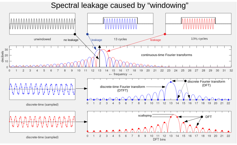
Different window functions introduce different amounts of scalloping noise/artifacts. Scalloping noise occurs when the frequency bins of a DFT don't optimally align with the DTFT.

The shape of the DTFT corresponds to the Fourier transform of the window function, and thus window functions whose Fourier transform has shorter side-lobes will have less scalloping noise. However, window functions with less scalloping noise are narrower in the time domain (the Rectangular window has the most scalloping noise) and thus, without window overlapping, will lose the frequencies at the edges of the window.

Terminology

Since the frequency content of overlapping windows are displayed sequentially rather than averaged, I find talking about overlapping windows confusing. I would rather divide the time domain into Frames for which we try to obtain a picture of the frequencies in their range as accurately as possible. This may involve extending the window function past the range of the frames to minimize the scalloping noise/windowing loss tradeoff. However, this will introduce leakage of the frequencies between neighboring frames (reducing time resolution).

Window lengths and sample rates

Edit: My answer here was bad and I replaced it with this:

Frequency resolution is how similar the window function's magnitude in frequency space is to the Dirac delta function. This is because the product of the window and the signal in the time domain becomes convolution in the frequency domain (and a convolution with the Dirac delta function is a sampling which would give perfect frequency resolution) The fatter the mainlobe (quantified by it's variance), and the higher the sidelobes, the worse the frequency resolution. Additionally, Time resolution can be quantified a the variance of the window function in the time domain.

From wikipedia https://en.wikipedia.org/wiki/Short-time_Fourier_transform#Resolution_issues:

The product of the standard deviation in time and frequency is limited. The boundary of the uncertainty principle (best simultaneous resolution of both) is reached with a Gaussian window function, as the Gaussian minimizes the Fourier uncertainty principle.

The key to note is that Praat's Gaussian Window is twice as long as it's other window functions. In the STFT you can extend you can have an extremely long window function compared to the time interval you want a view of the frequencies for, so long as the window function is close enough to zero for outside of your desired interval. This is optimal. Use the adjustable windows https://en.wikipedia.org/wiki/Window_function#Adjustable_windows

Zero padding

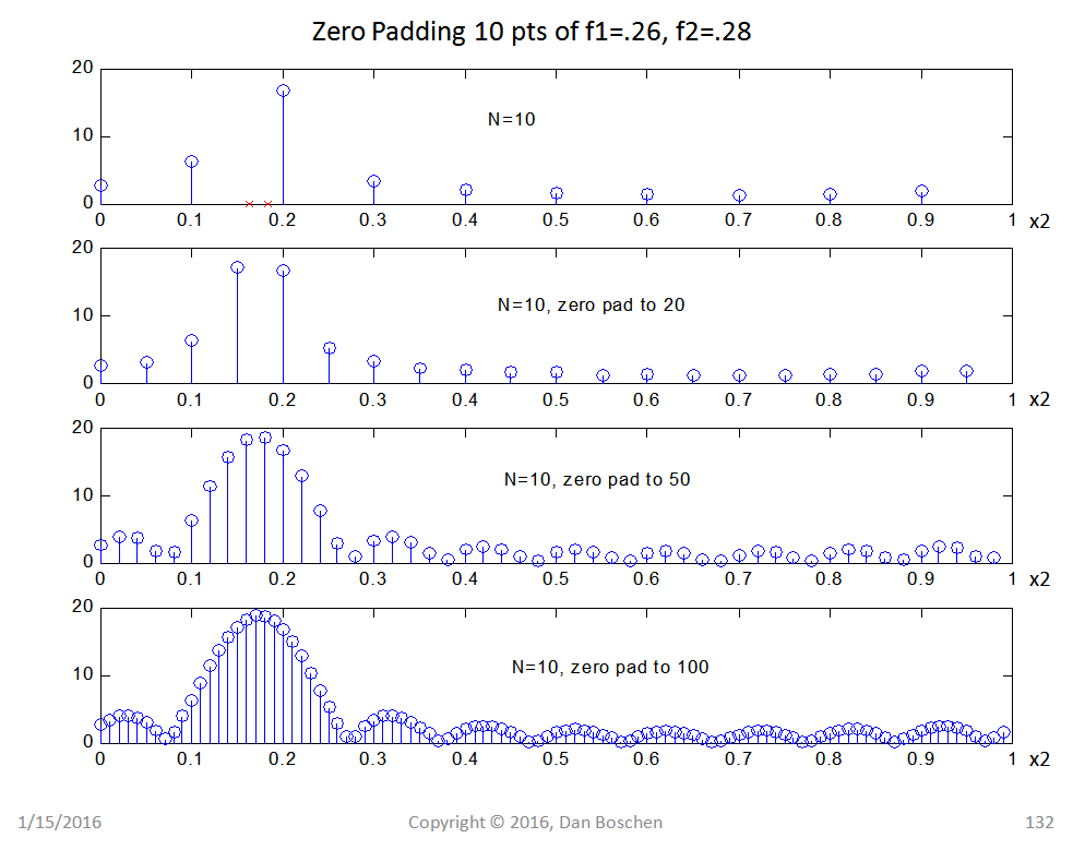
Zero padding doubles the number of bins while keeping the maximum frequency the same, interpolating the DTFT:

From Dan Boschen's answer What happens when N increases in N-point DFT