Computationally Efficient Ways of Determining If Pixels Are Clumped

Question

I'm working on an application where I get a video frame that's already segmented into good and bad pixels (as in -- the hardware either coughs up a pixel value or a flag that says "bad"). I want to come up with a figure of merit for the frame that's based both on the number of bad pixels and the amount that they are clumped, with one big clump being worse than a bunch of little ones.

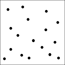
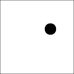
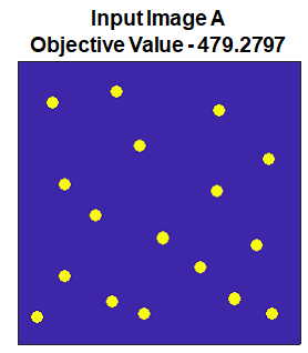
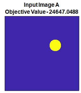
Here's two pictures to illustrate: the left picture has 17 dots 10 pixels in diameter -- it's better, on the theory that the dots are artifacts that can be "seen around". The right picture has about the same number of bad pixels, but they're all in one dot 41 pixels in diameter -- it's worse, on the theory that having so many bad pixels in a clump may occlude something interesting.

Things I can think to do:

• Walk the perimeter of each clump (really inefficient)
• Low-pass filter (originally I was thinking to use an FFT and look for high frequency content (not terribly efficient, and not terribly accurate, either, I think))
• draw a box around the bad pixels by finding the largest vertical and horizontal extents, and compare the area of that box to the bad pixel count (this could have false negatives if there's a large blob and a few little dots)

Are there known good ways to do this?

Answer 1

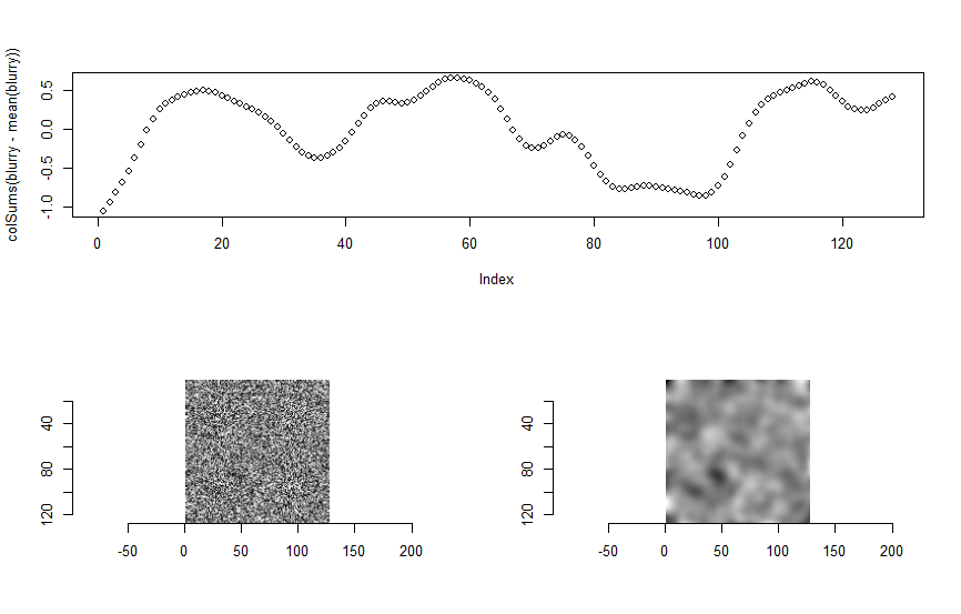
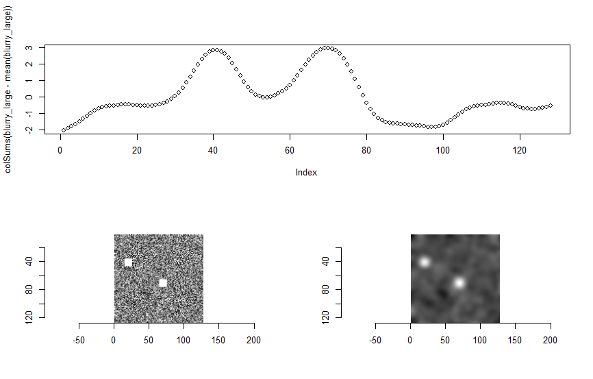
I've not tried this, but I'm wondering if something like a simple low pass filtering, followed by a column sum will do.

No time to explain code right now, but this seems to do something like what you want. Will return in a few hours and explain what it's doing.

---

R Code Below

library(imager)

N <- 128

noise <- array(runif(N*N*1*1),c(N,N,1,1)) #5x5 pixels, 1 frames, 1 colours. All noise
small_clumps <- as.cimg(noise)
blurry <- isoblur(small_clumps,5)

layout(matrix(c(1,1,2,3), 2, 2, byrow = TRUE))
plot(colSums(blurry-mean(blurry)))
plot(small_clumps)
plot(blurry)


large_clumps <- small_clumps
large_clumps[65:75, 65:75] <- 1
large_clumps[15:25, 35:45] <- 1
blurry_large <- isoblur(large_clumps,5)
# par(mfrow=c(3,1))
layout(matrix(c(1,1,2,3), 2, 2, byrow = TRUE))
plot(colSums(blurry_large-mean(blurry_large)))
plot(large_clumps)
plot(blurry_large)

Answer 2

Median filter? Use it to «thin out» bad pixels that appear locally sparse (for some definition of «local»). Then count the remaining bad pixels.

Or convolve with a large-ish 2d kernel (eg flat rectangular window) and decimate to get a number for «how many bad pixels are there inside each eg 16x16 window». Then accumulate the score for each block in a nonlinear fashion (so as to punish really dense blocks).

Im = randi([0 1], 640, 480);

Im_lp = conv2(ones(16), Im);

Im_lp_dec = Im_lp(8:16:end, 8:16:end);

score = sum(Im_lp_dec(:).^2);

Answer 3

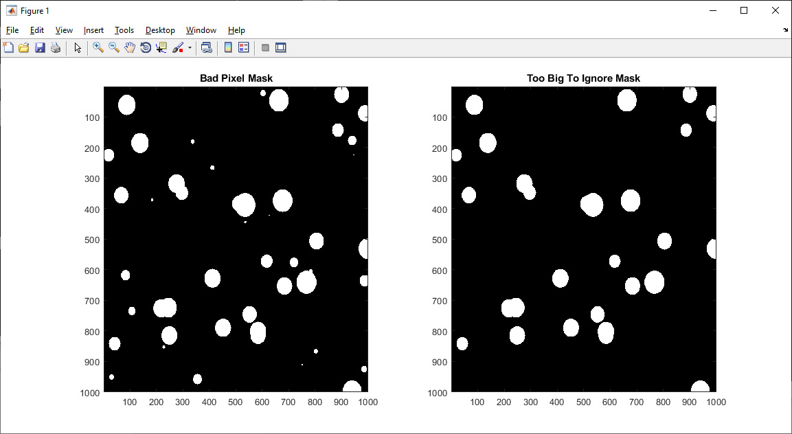
Erode the image using a structuring element which is the size/shape of the maximum allowable "bad region". Then dilate using the same structuring element. This will remove the bad-but-good-enough regions. From there you can work on characterizing/measuring what's left. Example given below using Matlab.

% Create a blank image.
Mimg = 1000;
Nimg = 1000;
img = zeros( Mimg, Nimg );

% Make up some coordinates.
m = 0 : Mimg - 1;
n = 0 : Nimg  - 1;
[ MM, NN ] = ndgrid( m(:), n(:).' );

% Populate the bad pixel mask.
Ncirc = 50;
dmax = 40;                              % Max possible radius
r = randi( dmax, [ Ncirc, 1 ] );        % Radius of circles
x0 = randi( Mimg, [ Ncirc, 1 ] ) - 1;   % x-coorindate of center
y0 = randi( Mimg, [ Ncirc, 1 ] ) - 1;   % y-coordinate of center
for ii = 1 : Ncirc 
  t = sqrt( ( x0(ii) - MM ).^2 + ( y0(ii) - NN ).^2 );
  img( t <= r(ii) ) = 1;
end

% The threshold radius for unignorable bad regions.
d = 20;

% Create the structuring element.
s = sqrt( bsxfun( @plus, ( (1:d*2)' - d ).^2, ( (1:d*2) - d ).^2 ) ) <= d;

% Remove the bad pixel regions that are too small to care about.
img_bad = imdilate( imerode( img, s ), s );

figure();
set( gcf(), 'color', 'w' );
subplot( 1, 2, 1 );
imagesc( img );
colormap( gray );
title( 'Bad Pixel Mask' );
subplot( 1, 2, 2 );
imagesc( img_bad );
title( 'Too Big To Ignore Mask' );
colormap( gray );

Answer 4

The approach I took was using MATLAB's functions, either regionprops() or bwconncomp() and bwdist().

The idea is to give a grade for each pixel which is a part of bad pixels object.
The grade is the radius of the circle bounding the object the pixel resides in.

One way to calculate the radius of the bounding circle is the MajorAxisLength property in the output of regionprops().
Another nice trick is using the Binary Image Distance Transform. If you apply the distance transform to the image where each bad pixels is black and the rest of the pixels is white, then for each object the maximum value represents the radius of the bounding image and the coordinate represent the center of the bounding circle.

So for pixel I gave a grade and then summed the value of all pixels.
The result is as expected:

The score above completely ignores the content of the frame and only takes into account the map of the bad pixels.
In real world application I'd do one extra step. I would take Saliency Map into account. Then for pixels which are in an important location I'd add more to their score.

The full MATLAB code is available on my StackExchange Signal Processing Q63549 GitHub Repository (Look at the SignalProcessing\Q63549 folder).