1
$\begingroup$

I have accelerometer [x,y,z] data recorded from various activities. I am not looking at any filtering techniques (which I have seen within this forum) because I want to be able to measure the amplitude of the noise for each activity sample set using a global time-domain feature average loudness.

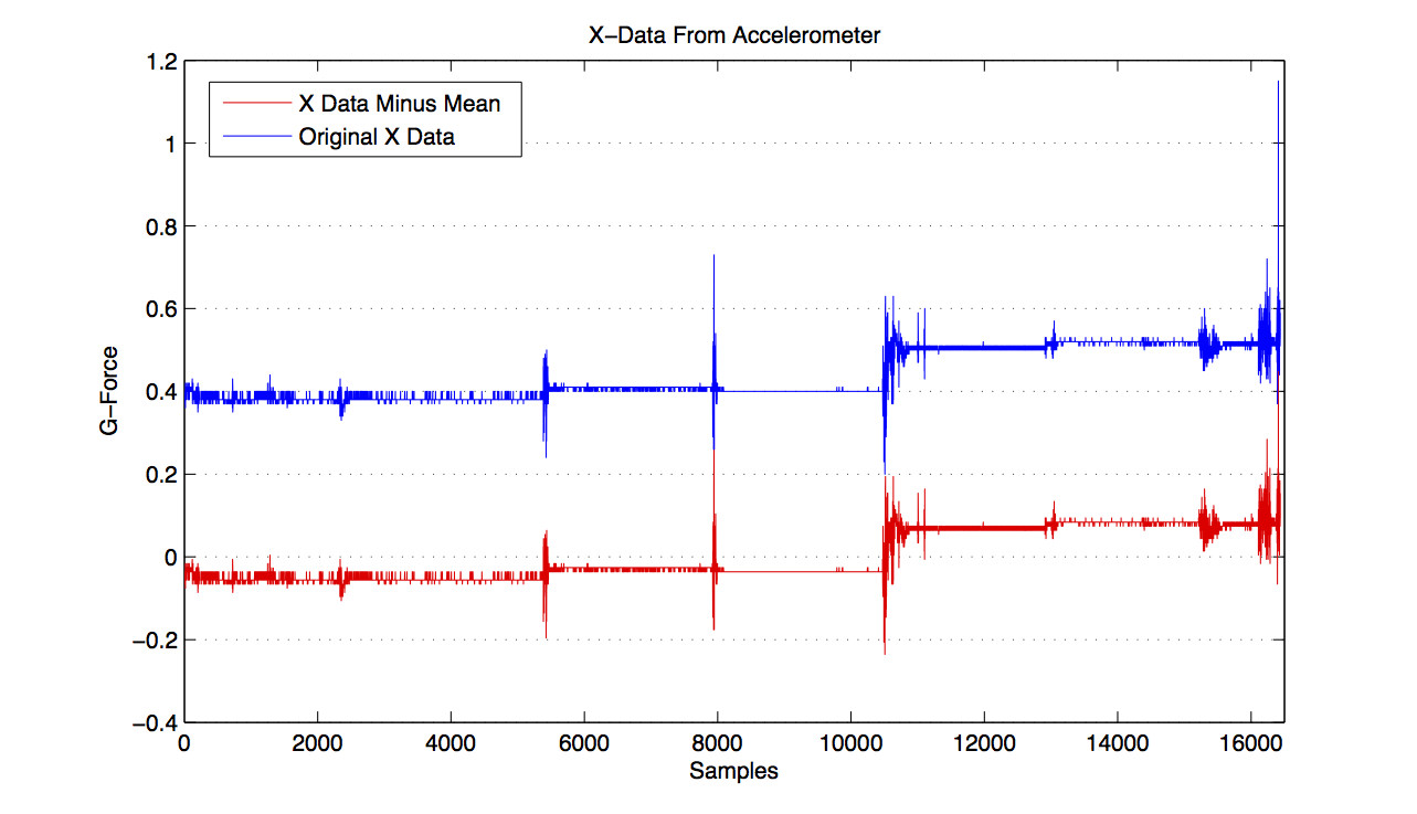
I am curious to know if I can center the signal around 0g, similarly to the X Data Minus Mean vector plot, but without the x-axis orientation i.e. the signal shifting up and down?

I have the x-axis data from one of my activities below:

ACCEL

I was hoping that by subtracting the mean from the x-axis data would yield this, but all it has done is shifted the entire signal down to around 0g.

The reason I ask is because I am unsure if computing a time-domain feature such as average loudness will work with the signal shifting up and down?

Average Loudness/Energy: AE

$\endgroup$

3 Answers 3

2
$\begingroup$

Your data is composed of a majoriy of low-activity regions, with higher-amplitiude sparse/concentrated activities. The bad news is that most of the methods to achieve your goal are likely to somehow filter your data. The good news is that non-linear filtering could help you.

If you are not concerned with calculations and real-time yet, I would suggest first a centered median filter to extract a robust $0 g$ estimate, and remove it from the data. In other words: choose an appropriate left-right span of $K$. In each window around index $k$, computes the signal $\hat{s}(k) = s(k) - \textrm{median} [s_{k-K},\ldots,s_{k+K}]$.

A median is a non-linear filter minimizing the $ell_1$ norm (like the $ell_2$ norm minimization yields the standard mean). It is somewhat robust to outliers, and since yours are both above and below your thought $0 g$ estimate, a running median (computed around each sample) could extract this 0-level reference.

Looking at your plots, start with $K=50,100,200$ to see if this starts to provides you with what you are looking for. Then, more involded techniques could be considered.

$\endgroup$
8
  • $\begingroup$ I see, so decompose my accelerometer data into non-overlapping frames of 50 samples or above, then take the median of a frame, then subtract that from each sample within the frame? I am not concerned with a high-level of accuracy, but I am hoping to see a difference in values when the accelerometer is fairly static to moving abruptly. $\endgroup$ Commented Oct 3, 2015 at 15:30
  • $\begingroup$ Thus, please use overlapping frames, for each $k$ index sample. Can you share your data? And do you use Matlab-like coding? $\endgroup$ Commented Oct 3, 2015 at 15:32
  • $\begingroup$ Yes I can share the data, and yes I use MatLab. I already have some code that lets you choose a window and hop size in samples or ms. This also uses a hamming window - is this needed? $\endgroup$ Commented Oct 3, 2015 at 15:40
  • $\begingroup$ So far, the window does not seem necessary to me, but could become useful as a weighhting for the filtering. Meanwhile, you can share them all to improve answers $\endgroup$ Commented Oct 3, 2015 at 15:50
  • $\begingroup$ Ok - do I perform this median operation on the original vector or the vector where I have subtracted the mean (the red plot)? $\endgroup$ Commented Oct 3, 2015 at 15:52
0
$\begingroup$

Your AE(x) equation sure looks like what I'd call the "average power" of a time sequence. And non-zero DC levels will influence that AE(x) value. But I have the impression you're trying to measure the energy in just the transient spikes of your signal and ignore the DC levels upon which those spikes are riding. If I'm correct, perhaps a "moving variance" estimation process would be useful. (Computing a "moving variance" is similar in concept to computing a "moving average".) If you e-mail me at R_dot_Lyons_@_ieee_dot_org I can send you some material on moving variance estimation. Then again, maybe just passing your signal through a digital differentiator will produce useful information. I'm just throwing out ideas here.

$\endgroup$
3
  • $\begingroup$ Yes, I am trying to get some form of energy estimate based on the transient spikes. Preferably a single statistic I can use to infer that somebody with an accelerometer strapped to them is somewhat static, to somebody who is moving around abruptly. I've just tried a median filter, but the trend mentioned below still exists. So a moving variance involves overlapping frames that instead of being averaged are being measured for variance i.e. using std(frame) within Matlab? I am also unsure what a digital differentiator is. $\endgroup$ Commented Oct 3, 2015 at 18:30
  • $\begingroup$ A digital differentiator is a kind of filter whose output estimates of the derivative of the input. A digital differentiator will detect abrupt changes in the input signal. Just to see what I’m talkin’ about here, in Matlab try this (assuming your input signal is variable ‘Sig’): B = [-1/16, 0, 1, 0, -1, 0, 1/16]; A = 1; % Dig. Diff. Differentiator_Out = filter(B, A, Sig); Rectified = abs(Differentiator_Out); AC_Energy = var(Rectified) figure(10), plot(Rectified) The AC_Energy value will be a single value proportional to the energy in the transient spikes of your original ‘Sig’ signal. $\endgroup$ Commented Oct 4, 2015 at 9:56
  • $\begingroup$ Thanks Richard, I will try this code in MatLab in order to understand this. Also sent the requested data in a .csv format earlier. $\endgroup$ Commented Oct 4, 2015 at 18:35
-1
$\begingroup$

The abrupt DC shifts appear like some trend. (Though off-topic, can I know what physical variation map to these DC shifts). As suggested previously, the problem can be circumvented, to certain extent, by using non-linear filtering. I can think about the following:

  1. Carry out an Empirical Mode Decomposition (EMD, matlab code available here: http://perso.ens-lyon.fr/patrick.flandrin/emd.html). EMD decomposes the signal into few intrinsic mode functions (IMFs). When you add all the IMFs you get back the original signal. The key in the decomposition is the notion of data dependent filtering, and the last few IMFs capture the slow varying signal trend. Hence, I will suggest you do an EMD and discard the last few IMFs, and see the resulting summed up signal.
  2. Differentiation: As suggested above but take care to choose your finite difference operation appropriately, else it may blow up the noise transients as well.
  3. Though you are not willing to do this, I will still suggest, the average loudness here will refer to the high frequency spectrum energy content.This is implicitly what you will be obtaining from option 1 and 2.
$\endgroup$
1
  • $\begingroup$ Any clarification for -1? :-| $\endgroup$
    – Neeks
    Commented Oct 4, 2015 at 13:05

Your Answer

By clicking “Post Your Answer”, you agree to our terms of service and acknowledge you have read our privacy policy.

Not the answer you're looking for? Browse other questions tagged or ask your own question.