The explanation given in your text is, unfortunately, quite dreadful
and confuses several issues. We have a low-pass function $x(t)$ whose sample values $$\cdots, x((n-2)T), x((n-1)T), x(nT), x((n+1)T), \cdots$$
are given to us. Note the complete absence of any subscript $a$ on $x$.
We write $x_n$ for the $n$-th sample value $x(nT)$. We wish to reconstruct $x(t)$ from its samples, and our reconstruction
is $x_a(t)$ as (incorrectly) defined in (1.4.23): the correct
definition is
$$x_a(t) = \sum_{n=-\infty}^\infty x(nT)g(t-nT)
= \sum_{n=-\infty}^\infty x_n g(t-nT).\tag{1.4.23.corrected}$$
Note again the complete absence of any subscript $a$ in
the middle sum, and the right-hand sum emphasizes that the reconstruction
is a weighted sum of delayed versions of $g(t)$ with the weights
being the given sample values.
The function $x_a(t)$ as
defined in $(1.4.23.\text{corrected})$ has the property that if $t=mT$,
then
$$x_a(mT) = \sum_{n=-\infty}^\infty x_ng(mT-nT)
= \sum_{n=-\infty}^\infty x_n g((m-n)T) = x_m \tag{1}$$
because $g(t)$ is a Nyquist pulse and enjoys the property
that $g(\ell T) = 0$ if $\ell$ is a nonzero integer while
$g(0) = 1$. Thus, the reconstructed function $x_a(t)$ has
the property that at each sampling instant $mT$, the value of
$x_a(t)$, viz. $x_a(mT)$ equals $x_m$, the $m$-th sample
value given to us. Thus, as far as samples are concerned
the two functions $x_a(t)$ and $x(t)$ have the same values
at the sampling instants $mT$. In other words,
$$x_a(t) = x(t) \quad \text{for} \quad t = mT, m \in \mathbb Z.\tag{2}$$
Note that $(2)$ holds regardless of what $T$ is and how it
relates to the maximum frequency in $x(t)$ etc.
What at time instants other than multiples of $T$? Is it
true that $x_a(t)$ as defined in $(1.4.23.\text{corrected})$ equals
$x(t)$ for all $t, -\infty < t < \infty$?
Well, that is where the fun statrts. If the Nyquist criterion is met, then $x_a(t)$ as given in $(1.4.23.\text{corrected})$ is precisely
the $x(t)$ that we wish to recover. I will not prove this statement
(which is called the Nyquist theorem or the Shannon-Whittaker
sinc interpolation formula etc) but that $x_a(t)$ as defined
in $(1.4.23.\text{corrected})$ is $x(t)$ is what the crux of
the matter is. If the Nyquist criterion is
not met, then $(1.4.23.\text{corrected})$ gives a function $x_a(t)$
whose sample values
$x(t)$ at the sampling instants $mT$ (cf. the remarks surrounding
$(1)$ and $(2)$ above) but is not equal to $x(t)$
at other times. In fact, $x_a(t)$ is the result of aliasing
of $x(t)$ with respect to the sampling frequency etc, but that
is a matter for a different question.
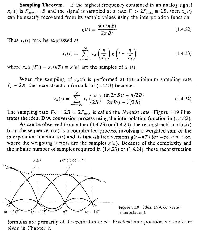
With that as preliminaries, let us turn to the illustration that
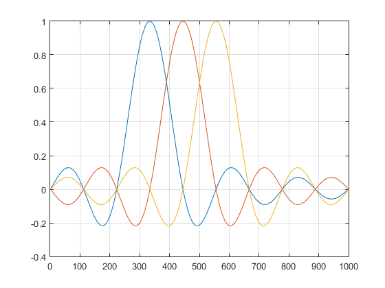
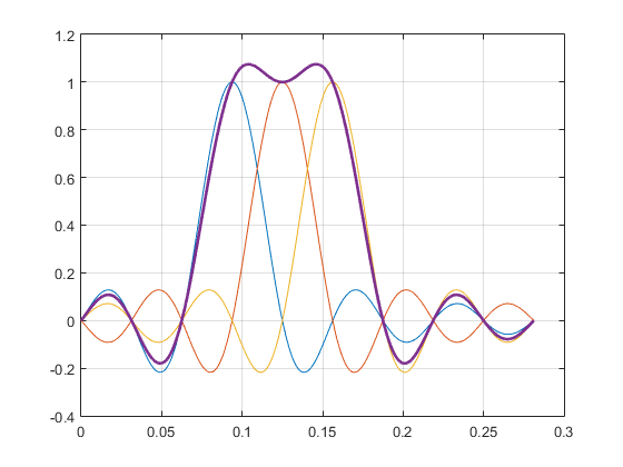
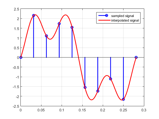
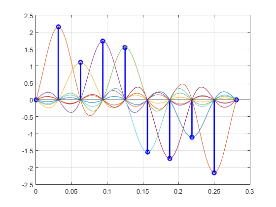
puzzles you. The dashed curve is the result of the interpolation:
the function
$x_a(t)$ as defined in $(1.4.23.\text{corrected})$ and it is
the sum of infinitely many weighted and delayed sinc functions.
The other curves are (four of the)
infinitely many sinc functions $x_m g(t-mT)$ on the right side
of $(1.4.23.\text{corrected})$. At $t=nT$, the term $x_ng(t-nT)$
which occurs on the right side of $(1.4.23.\text{corrected})$
has a peak value of $$x_ng(nT-nT) = x_ng(0) = x_n$$ and it has
value $0$ at other sampling instants
$\cdots, (n-2)T, (n-1)T, (n+1)T, \cdots$ Similarly, the function
$x_{n-1}g(t-(n-1)T)$ has value $x_{n-1}$ at $t=(n-1)T$ and value
$0$ at all other sampling instants. In short, if we evaluate the sum
$$\sum_{m=-\infty}^\infty x_m g(t-mT)$$
at $t=nT$, that sum of infinitely many terms simplifies
to $x(nT)$ because all
the other terms are $0$. No muss, no fuss, no worries about
convergence of an infinite series etc. Remember that
all this holds without any
issues of Nyquist criteria etc. The hard part is the assertion
that $x_a(t)$ as defined in $(1.4.23.\text{corrected})$ equals
$x(t)$ for all $t$ if the Nyquist criterion is satisfied.
So why all this yelling and screaming about (1.4.23) being incorrect
and the explanation in the text being sheer nonsense? Well,
(1.4.23) as shown in the OP's text has sample values of $x_a(t)$,
the reconstructed signal, on the right side. So, the definition
is circular, to say the least, and even if we ignore that, it
is an assertion of the Nyquist theorem or the Shannon-Whittaker
interpolation formula without any proof. The equality
(1.4.23) as given in the text holds at $t=mT, m \in \mathbb Z$;
the assertion that it holds for all $t$ is a proof by intimidation.
 (Image source: Digital Signal Processing Principles Algorithms and Applications)
