Why is my discretized transfer function unstable when my discretized state-space model is stable?

Question

I am working with a 30-state, 14-input linear model that is described by a state-space model:

model_state_space = ss(A, B, C, D);

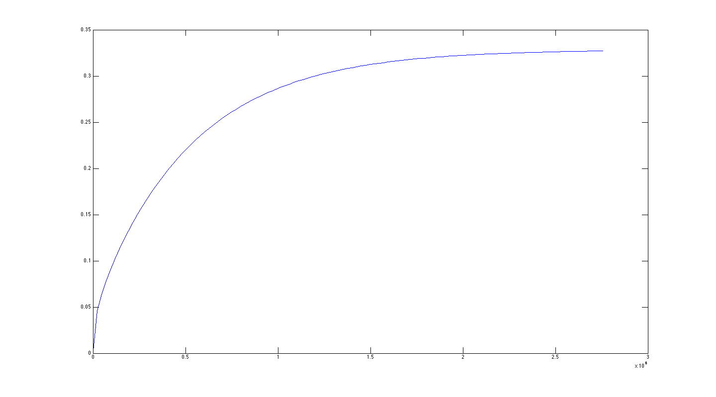
The model is extremely slow (it describes the thermal behavior of a building), so when I discretize it I choose a sample time of 900 seconds and plot the step response from one of the inputs:

[y,t] = step(model_state_space);
plot(t, y(:,:,end))

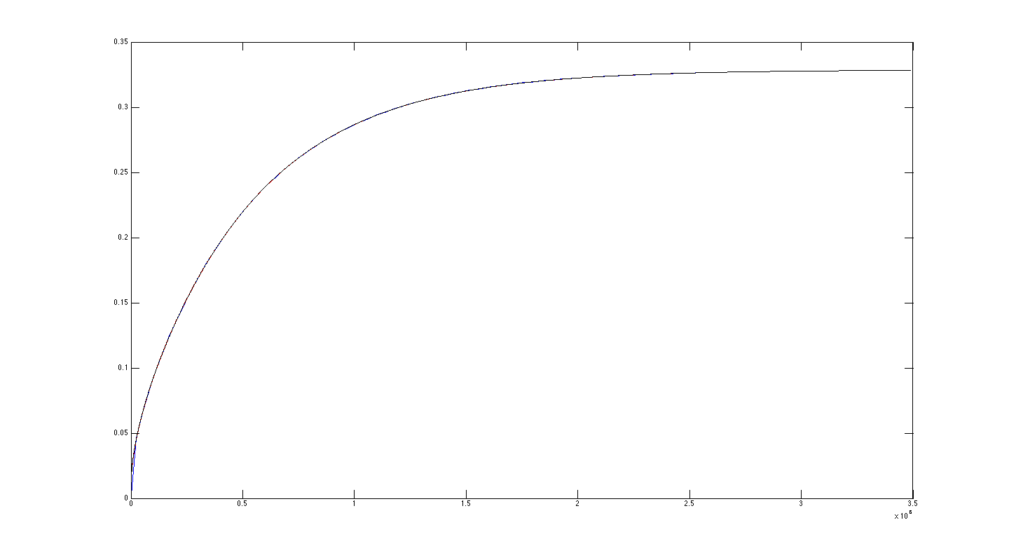
I obtain a similar plot when I compute the step response of the discretized state-space model, or of the equivalent transfer function continuous model:

hold on
[y,t] = step(c2d(model_state_space, 900));
plot(t,y(:,:,end), 'r')
[y,t] = step(tf(model_state_space));
plot(t,y(:,:,end), 'k')

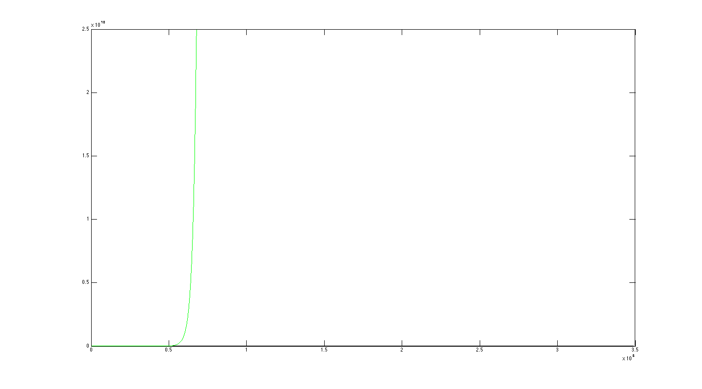
But when I compute the impulse response of the discretized transfer function, the system appears unstable:

[y,t] = step(c2d(tf(model_state_space), 900));
plot(t,y(:,:,end), 'g')

Can someone please explain why this is so?

Answer 1

You're using a high order model so you might be running into numerical precision issues.

Make sure the realization of model_state_space is minimal. You can do this with

min_model_state_space = minreal(model_state_space)

Also, not all state-space realizations are created equally. Some have better numerical properties, such as a balanced realization:

[balanced_model_state_space, G] = balreal(model_state_space)

If the vector G contains small values it means you can reduce the order of your model without giving up accuracy. Look up the matlab function balred.

Just from looking at your step response plot you probably don't need a 30th order model (1st or 2nd order might even be enough).

Answer 2

I found a thread on MATLAB Central that deals with exactly this problem: http://ch.mathworks.com/matlabcentral/newsreader/view_thread/7746