java resampling implementation using sinc function

Question

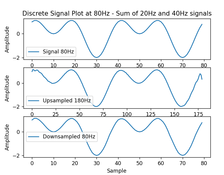
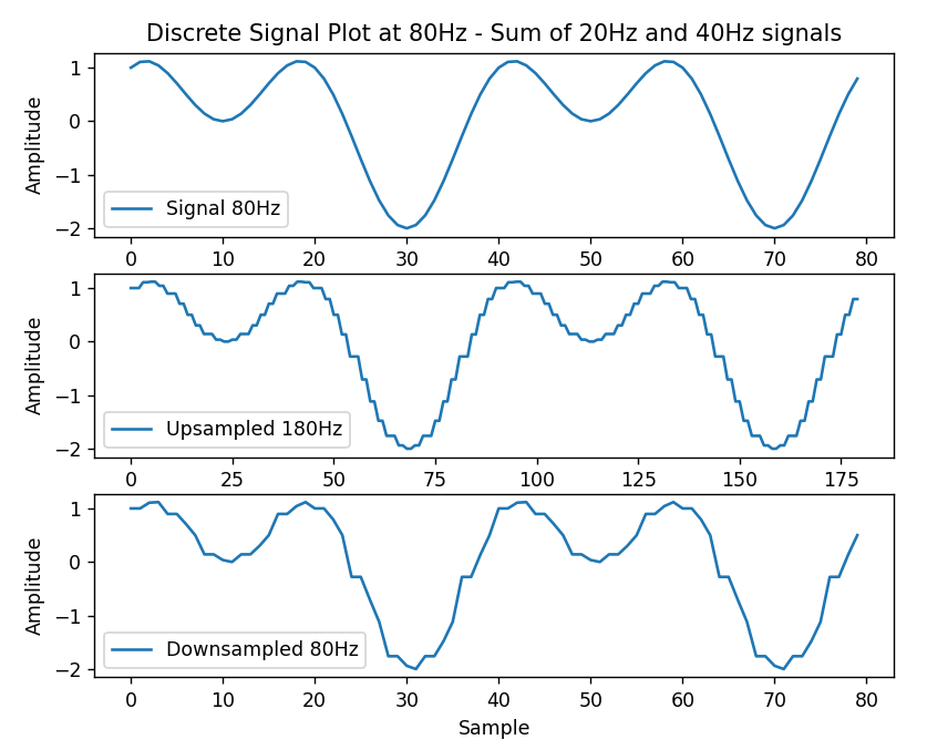
To be as succinct as possible, I've written a Java method that implements resampling of a signal using the sinc function interpolation formula. When I test this code with a simple sinusoid, I'm able to take a test signal, upsample it, downsample it back to the original frequency, and it comes out identical. Perfect! Then when I test it with a 10 second audio wav file, it totally borks. In my successful test, the input is a 20Hz sine + 40Hz cosine which I sample at 80Hz, then upsample to 180Hz, then downsample back to 80Hz. For the audio file, its a mono 44.1khz sample which I downsample to 16kHz. Here's the code, then I'll paste the formula I've implemented (maybe I've got the formula wrong).

/**
 * Calculates an interpolated value when resampling - THIS IS THE MAGIC!
 * This method is used to calculate the M sample of the output signal, given the input signal.
 * We don't necessarily need the entire input signal, but enough to encompass the window
 *
 * @param input        (Xi) the input signal
 * @param inputFreq    (Fi) the input signal freqency
 * @param output_m     (M) the current sample number in the output signal we are calculating)
 * @param windowLength (L) we will evaluate the input signal in the window N-L to N+L
 * @param newfreq      (Fo) the output frequency
 * @return the interpolated value
 */
public static double interpolate(double[] input, int inputFreq, int output_m, int newfreq, int windowLength) {
    double sum = 0.0;
    double t_i = 1.0 / inputFreq;
    double t_o = 1.0 / newfreq;
    int    q   = (int) Math.floor(output_m * t_o / t_i); // this is the corresponding sampleNr in the input signal

    for (int n = -windowLength + q; n <= windowLength + q; n++) {
        // First handle edge conditions
        if (n < 0) // skip n < 0
            continue;
        if (n >= input.length) // EOF
            break;
        double mTo_minus_nTi_over_Ti = (output_m * t_o - n * t_i) / t_i;
        if (mTo_minus_nTi_over_Ti == 0)
            sum += input[n];
        else {
            double pi_times = Math.PI * mTo_minus_nTi_over_Ti;
            double sineterm = Math.sin(pi_times) / pi_times;
            double xi_n     = input[n];
            double sumterm  = xi_n * sineterm;
            sum += sumterm;
        }
    }

    return sum;
}

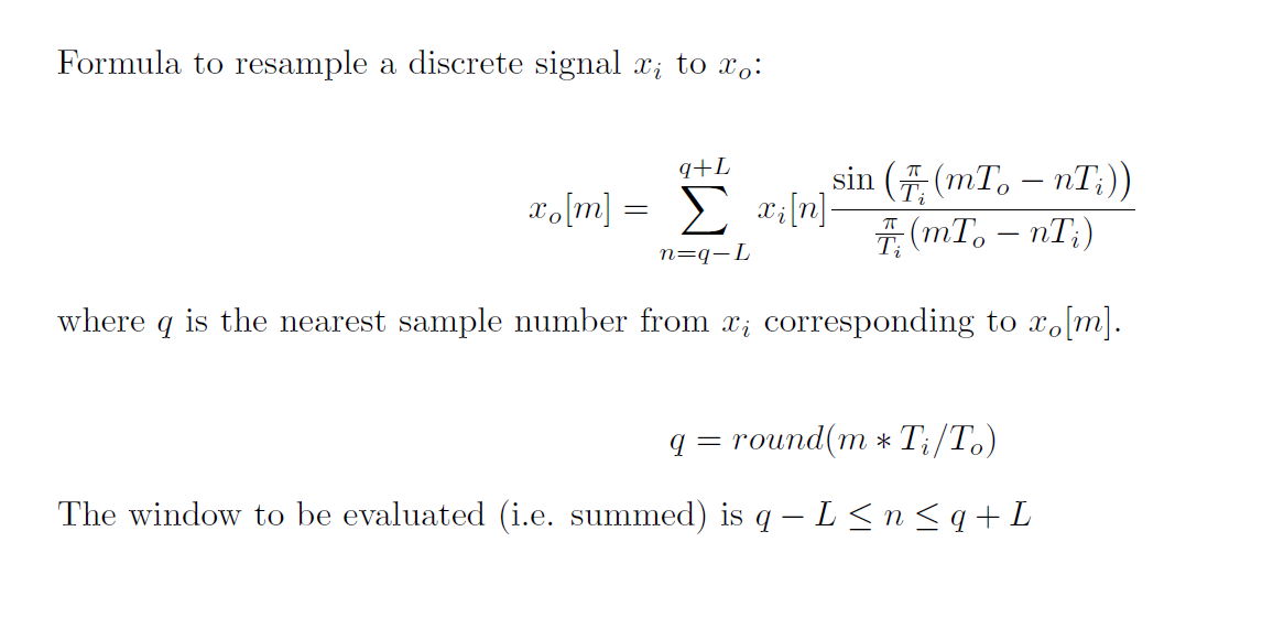
Here is the formula I used (I created this latex image to reflect what I implemented - please don't assume it's right, because if it is, I can't figure out where I've gone wrong! :) )

My simple visual test results:

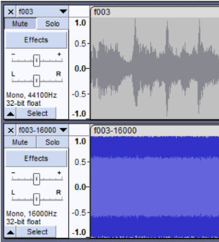
My visual audio test results - all noise and static:

Maybe my error above is obvious. I hope so! But I wondered, in the sinc function, is "n" supposed to be the sample number from the input, or is it supposed to be the fraction that leads to the nearest input sample number? So I made a couple of changes, leaving "q" and "n" as doubles, and only taking Math.floor of n when I need the actual sample number.

    public static double interpolate(double[] input, int inputFreq, int output_m, int newfreq, int windowLength) {
        double sum = 0.0;
        double t_i = 1.0 / inputFreq;
        double t_o = 1.0 / newfreq;
        double q   = (output_m * t_o / t_i); // this is the corresponding sampleNr in the input signal

        for (double n = -windowLength + q; n <= windowLength + q; n++) {
            // First handle edge conditions
            if (n < 0) // skip n < 0
                continue;
            if (n >= input.length) // EOF
                break;

            double mTo_minus_nTi_over_Ti = (output_m * t_o - n * t_i) / t_i;
            if (mTo_minus_nTi_over_Ti == 0)
                sum += input[(int) Math.floor(n)];
            else {
                double pi_times = Math.PI * mTo_minus_nTi_over_Ti;
                double sineterm = Math.sin(pi_times) / pi_times;
                double xi_n     = input[(int) Math.floor(n)];
                double sumterm  = xi_n * sineterm;
                sum += sumterm;
            }
        }

        return sum;
    }

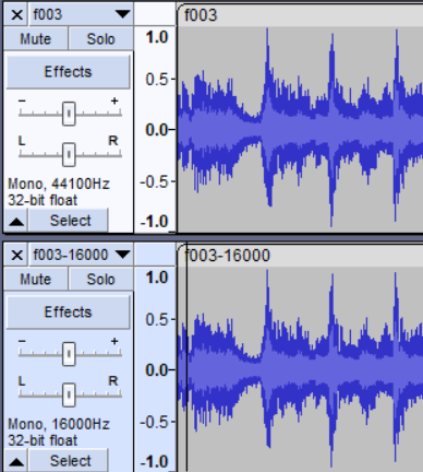
Suddenly, the audio resampling looks (and sounds) perfect!

But the sinusoid plot now looks like this, which is clearly not a perfect reconstruction. What's happening is that all of the interpolated samples are equal to the nearest direct sample, thus the horizontal artifacts.

Apologies for the long post, I tried to keep it concise and directed. Full disclosure - yes this is a school assignment, but this isn't for a DSP class, its actually a parallel computing class where we need to process very large audio files very fast! I've shared all of the above and the link to this post with the professor.

Thanks in advance for any help!

Answer 1

Try first to upsample your 41kHz file to e.g. 96kHz, and see if it works, if so, it may be related to aliasing.

Notice that when you do a sync interpolation what you are doing is to convolve the original signal with a $sinc(2 f_b t)$, where $f_b$ defines the bandwidth of the filtered signal, then you are sampling this continuous signal at times $t_k = k / f_s$, in order to avoid aliasing $f_s \le 2f_b$ is required. In your interpolation

$$x_o[n] = \sum x_i[m] \, sinc\left(m \frac{T_o}{T_i} - n\right)$$

This conditon is satisfied when upsampling but not when downsampling.

A simple change to adjust the bandwidth accordingly to the output sampling frequency would be

$$x_o[n] = \sum x_i[m] \, sinc\left(m - \frac{f_o}{f_i} n\right)$$

I will use python to illustrate, note that I am plotting using your interpolation formula.

The described signal

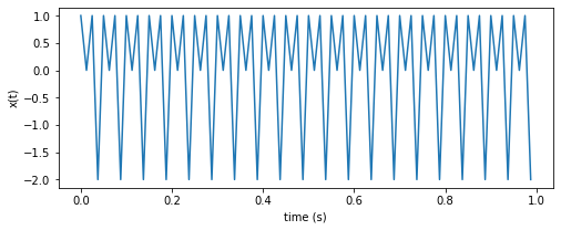
the input is a 20Hz sine + 40Hz cosine which I sample at 80Hz,

Such signal should look like this

import numpy as np
import matplotlib.pyplot as plt

# sample time at 80Hz
t80 = np.arange(0, 1, 1/80);
# curve
x80 = np.sin(20*2*np.pi*t80) + np.cos(40*2*np.pi*t80)
plt.figure(figsize=(8,3))
plt.plot(t80, x80);
plt.xlabel('time (s)')
plt.ylabel('x(t)')

That's not how your plot looks like

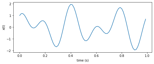
For a reference I will use a signal with 5Hz and 3Hz components.

# sample time at 80Hz
t80 = np.arange(0, 1, 1/80);
# curve
x80 = np.sin(3*2*np.pi*t80) + np.cos(5*2*np.pi*t80)
plt.figure(figsize=(8,3))
plt.plot(t80, x80);
plt.xlabel('time (s)')
plt.ylabel('x(t)')

The sinc interpolation

Here is a quick implementation of the resampling, the sinc_sample function works like your java function, given an output index, input, frequencies and L, it evaluates one sample.

The sinc_resample process the entire wave using sinc_resample, probably the operation you want to parallelize in your assignment.

def sinc_sample(x, m, f_in, f_out, L):
    q = m * f_in / f_out;
    qi = int(q)
    n = np.arange(max(0, qi-L), min(len(x), q+L+1), dtype=int);
    return np.sum(x[n] * np.sinc(q - n));

def sinc_resample(x, f_in, f_out, L):
    t = np.arange(0, len(x)/f_in, 1/f_out);
    return t, np.array([sinc_sample(x, m, f_in, f_out, L) for m in range(len(t))]);

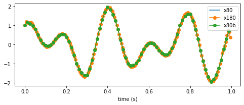
Interpolating a sufficiently smooth wave

In your example curve you start with something already smooth then you upsample from 80Hz to 180Hz, so it is a curve with a narrow spectrum.

x80 = np.sin(3*2*np.pi*t80) + np.cos(5*2*np.pi*t80)
plt.figure(figsize=(8,3))
plt.plot(t80, x80);
t180, x180 = sinc_resample(x80, 80, 180, L=3);
t80b, x80b = sinc_resample(x180, 180, 80, L=3);
plt.plot(t180, x180, '-o');
plt.plot(t80b, x80b, '-o');
plt.xlabel('time (s)')
plt.legend(['x80', 'x180', 'x80b'])

Nyquist limit

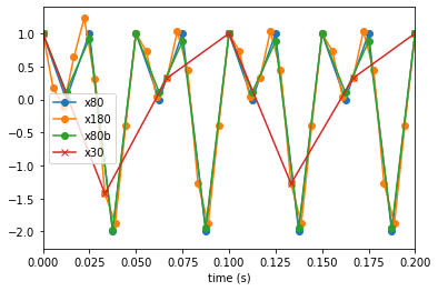
If you start from a 44kHz wave and downsample it to 16kHz, it is possible that the original wave has details, fast variations, that can't be described in 16kHz sampling. That's analogous to starting from 80Hz with frequencies close to the Nyquist limit and going to a lower frequency, e.g. 30Hz

x80 = np.sin(20*2*np.pi*t80) + np.cos(40*2*np.pi*t80)
plt.plot(t80, x80, '-o');
t180, x180 = sinc_resample(x80, 80, 180, L=3);
t80b, x80b = sinc_resample(x180, 180, 80, L=3);
t30, x30 = sinc_resample(x80, 80, 30, L=3)
plt.plot(t180, x180, '-o');
plt.plot(t80b, x80b, '-o');
plt.plot(t30, x30, '-x');
plt.legend(['x80', 'x180', 'x80b', 'x30'])
plt.xlabel('time (s)')
plt.xlim(0, 0.2)

Notice that the red line does not closely follow the other lines.

Updating the sampling function

A simple change to the function would be

def sinc_sample2(x, m, f_in, f_out, L):
    q = m * f_in / f_out;
    qi = int(q)
    n = np.arange(max(0, qi-L), min(len(x), q+L+1), dtype=int);
    return np.sum(x[n] * np.sinc((q - n)*(f_out/f_in)));

and of course, you can rearrange the calculations to reduce the number of operations.