0
$\begingroup$

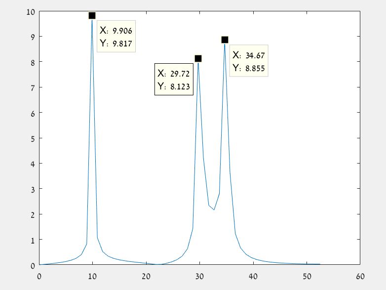
Hello i am trying to create the folding phenomena of undersampling in matlab, When i undersample the sampling frequency is 135 less than the Nyquist frequency for 70 Hz signal ou will see that it is shifted back by the amount of this new sampling frequency (105-70=35) Hz. as shown in the matlab plot bellow. I want to create the folding effect shown in diagram bellow (shifted copy). Where did i go wrong. This is my code which producedthe plot in the first post. my code is shown as one line for some reason.

f1=10;
f2=30;
f3=70;
% twice the sampling rate
Fs=1.5*70; % sampling frequency is a bit above 2 times to get all the peaks.
Ts=1/Fs;
Tn=0:Ts:1;
fft_L=length(Tn);
y4_samples=10*sin(2*pi*f1*Tn)+10*sin(2*pi*f2*Tn)+10*sin(2*pi*f3*Tn);
%stem(Tn_new,y4_samples);
ff=fft(y4_samples);
ff1 = abs(ff/fft_L);
fft2 = ff1(1:floor(fft_L/2)+1);
fft2(2:end) = 2*fft2(2:end);
f = Fs*(0:fft_L/2)/fft_L;
plot(f, fft2)

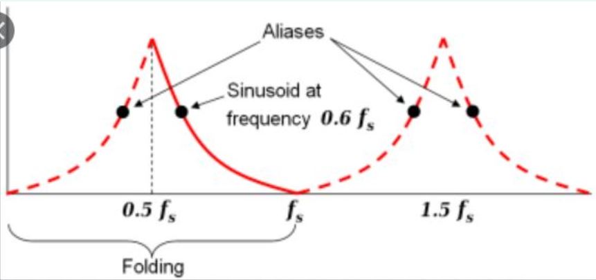
the effect i am looking for my matlab code

$\endgroup$
2
  • $\begingroup$ Can you post your code? What do you mean - the Nyquist frequency is $F_N = F_s/2$. $\endgroup$
    – teeeeee
    Commented Apr 2, 2020 at 8:43
  • $\begingroup$ This is my code which producedthe plot in the first post. f1=10; f2=30; f3=70; % twice the sampling rate Fs=1.5*70; % sampling frequency is a bit above 2 times to get all the peaks. Ts=1/Fs; Tn=0:Ts:1; fft_L=length(Tn); y4_samples=10*sin(2*pif1*Tn)+10*sin(2*pif2*Tn)+10*sin(2*pi*f3*Tn); %stem(Tn_new,y4_samples); ff=fft(y4_samples); ff1 = abs(ff/fft_L); fft2 = ff1(1:floor(fft_L/2)+1); fft2(2:end) = 2*fft2(2:end); f = Fs*(0:fft_L/2)/fft_L; plot(f, fft2) $\endgroup$
    – rocko445
    Commented Apr 2, 2020 at 9:43

2 Answers 2

2
$\begingroup$

Your plot is correct. You are sampling three waves $f_1 = 10\textrm{Hz}, f_2 = 30\textrm{Hz}$, and $f_3 = 70\textrm{Hz}$, with a sample frequency of $F_s = 1.5\times70\textrm{Hz} = 105\textrm{Hz}$. This means that your Nyquist frequency is $F_N = F_s/2 = 52.5\textrm{Hz}$, and corresponds to the maximum value of your frequency axis.

As such, the signals $f_1$ and $f_2$ will be correctly sampled without problems, but the signal $f_3$ is higher than the Nyquist and so should appear as an alias (folded back into the sampled frequency range) at the frequency $f_{\textrm{alias}} = F_N-(f_3-F_N) = F_s-f_3 = 35\textrm{Hz}$. This is what you obtained.

If you want to create a plot similar to the one in the figure, then you could try to first sample your waves with a much higher sampling rate, in order to fully capture them all faithfully. Then, on the same plot, display what happens if you undersample with $F_N<f_3$.

$\endgroup$
3
  • $\begingroup$ Hello as you said when i put f1=10 f2=20 f3=70 i get an alised harmonics at 35Hz but my 70Hz hamonics dissapears. Why is that? and How can we predict the amplitude of the harmonics? Thanks $\endgroup$
    – rocko445
    Commented Apr 2, 2020 at 10:23
  • $\begingroup$ As I said, if your Nyquist is only $52.5\textrm{Hz}$, you can never recover the wave at frequency $70\textrm{Hz}$, because it is outside your Nyquist and so it is greater than the maximum value you have on your frequency axis. Like I said in the answer, I would try repeat the process for a much higher sample rate as well (so you get the harmonic correctly), and plot them on the same graph. $\endgroup$
    – teeeeee
    Commented Apr 2, 2020 at 10:31
  • $\begingroup$ Try to gradually increase the frequency of $f_3$, start with $40\textrm{Hz}$, then $45\textrm{Hz}$, $50\textrm{Hz}$, etc. You will see that when you hit the Nyquist $52.5\textrm{Hz}$ and above then the peak will bounce back inside the band - this is the folding you were talking about. $\endgroup$
    – teeeeee
    Commented Apr 2, 2020 at 10:39
1
$\begingroup$

Your plot showing aliasing is applicable to complex signals.

You can emulate this exactly if you use:

y4_samples=10*e^(j*2*pi*f1*Tn)+10*e^(j2*pi*f2*Tn)+10*e^(j*2*pi*f3*Tn);

Note that real signals such as $\cos(2\pi f_1 T_n)$ actually consist of two complex frequencies as given by Euler's identity:

$$\cos(2\pi f_1 Tn) = \frac{e^{j2\pi f_1Tn} + e^{-j2\pi f_1 T_n}}{2}$$

This leads to the conclusion that aliasing for a signal $f$ with $f_N<f<f_s$ is given as $f_{alias} = 2f_n-f$ but that only applies to real signals where all frequencies are given as positive quantities. The general form that is applicable for all signals (just take absolute value to represent the real signals) is:

$$f_{alias} = mod(f, f_s) - f_N$$

Where

$f_{alias}$: aliased frequency in the first Nyquist zone $-f_s/2$ to $+f_s/2$

$f_s$: sampling frequency

$f$: frequency of signal getting sampled

So for real signals this would be:

$$f_{alias} = |mod(f, f_s) - f_N|$$

For signal processing in general where complex signals may be used this is a very important concept to understand; the aliasing actually rolls around from the highest frequency to the lowest rather than "folds" as is often described for real signals. For example, in your plot showing aliasing, the lower aliased frequency specifically is the one that maps to the lower frequency within the sampling bandwidth- this is in contrast to what you would conclude from a "folding" explanation.

$\endgroup$
7
  • $\begingroup$ from theory our data replicates in the range of [-pi,pi] $\endgroup$
    – rocko445
    Commented Apr 4, 2020 at 15:42
  • $\begingroup$ Yes that is consistent with what I am saying (for a normalized radian frequency of a complex signal). Here $f_N = \pi$ and $f_s = 2\pi$ so for a complex signal $f_{alias} = mod(f,f_s)-\pi$ so in the range of $[-\pi, \pi]$ but for a real signal $f_{alias} = |mod(f,\pi)-\pi|$, right? $\endgroup$ Commented Apr 4, 2020 at 15:44
  • $\begingroup$ Hello i cant see the logics of the vector "f" which represent our frequency domain. its supposed to be between [-pi,pi] but its not ,code start: ff1 = abs(ff/fft_L); fft2 = ff1(1:floor(fft_L/2)+1); f = Fs*(0:fft_L/2)/fft_L; plot(f, fft2); $\endgroup$
    – rocko445
    Commented Apr 4, 2020 at 15:53
  • $\begingroup$ It is because your f is given in terms of your sampling rate $F_s$ which is also given in cycles/sec (Hz). The $\pi$ in your frequency range in the comment is the normalized radian frequency in units of radians/cycle. $\endgroup$ Commented Apr 4, 2020 at 15:58
  • $\begingroup$ You have N samples in the FFT representing the frequencies from $f_s(0:N-1)/N$ where $f_s$ is the sampling rate in Hz, thus each frequency is given in Hz. If you want the normalized radian frequency you would need to use $2\pi(0:N-1)/N$. $\endgroup$ Commented Apr 4, 2020 at 16:00

Your Answer

By clicking “Post Your Answer”, you agree to our terms of service and acknowledge you have read our privacy policy.

Not the answer you're looking for? Browse other questions tagged or ask your own question.