Finding zebra-like pattern in image (Detection of structured-light fringe centerline from photo)

Question

I'm working in a project where fringes are projected against a subject, and a photo is taken. The task is to find the centerlines of the fringes, which represent, mathematically, the 3D curve of intersection between the fringe plane and the subject surface.

The photo is a PNG (RGB), and former attempts used grayscaling then difference thresholding to get a black-and-white, "zebra-like" photography, from which it was easy to find the midpoint of each pixel column of each fringe. The problem is that, by thresholding and also by taking the mean height of a discrete pixel column, we're having some precision loss and quantization, which is not desired at all.

My impression, by looking at the images, is that the centerlines could be more continuous (more points) and smoother (not quantized) if they were detected directly from the non-thresholded image (either RGB or grayscale), by some statistical sweeping method (some flooding / iterative convolution, whatever).

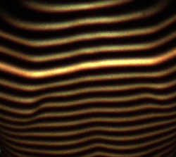
Below is an actual sample image:

Any suggestion would be much appreciated!

Answer 1

I suggest the following steps:

1. Find a threshold to separate the foreground from the background.
2. For each blob in the binary image (one zebra stripe), for each x, find the weighted center (by pixel intensity) in y direction.
3. Possibly, smooth the y values, to remove noise.
4. Connect the (x,y) points by fitting some kind of curve. This article might help you. You can also fit a high-level polynomial, though it is worse, in my opinion.

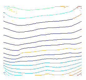
Here is a Matlab code that shows steps 1,2 and 4. I skipped the automatic threshold selection. Instead I chose manual th=40:

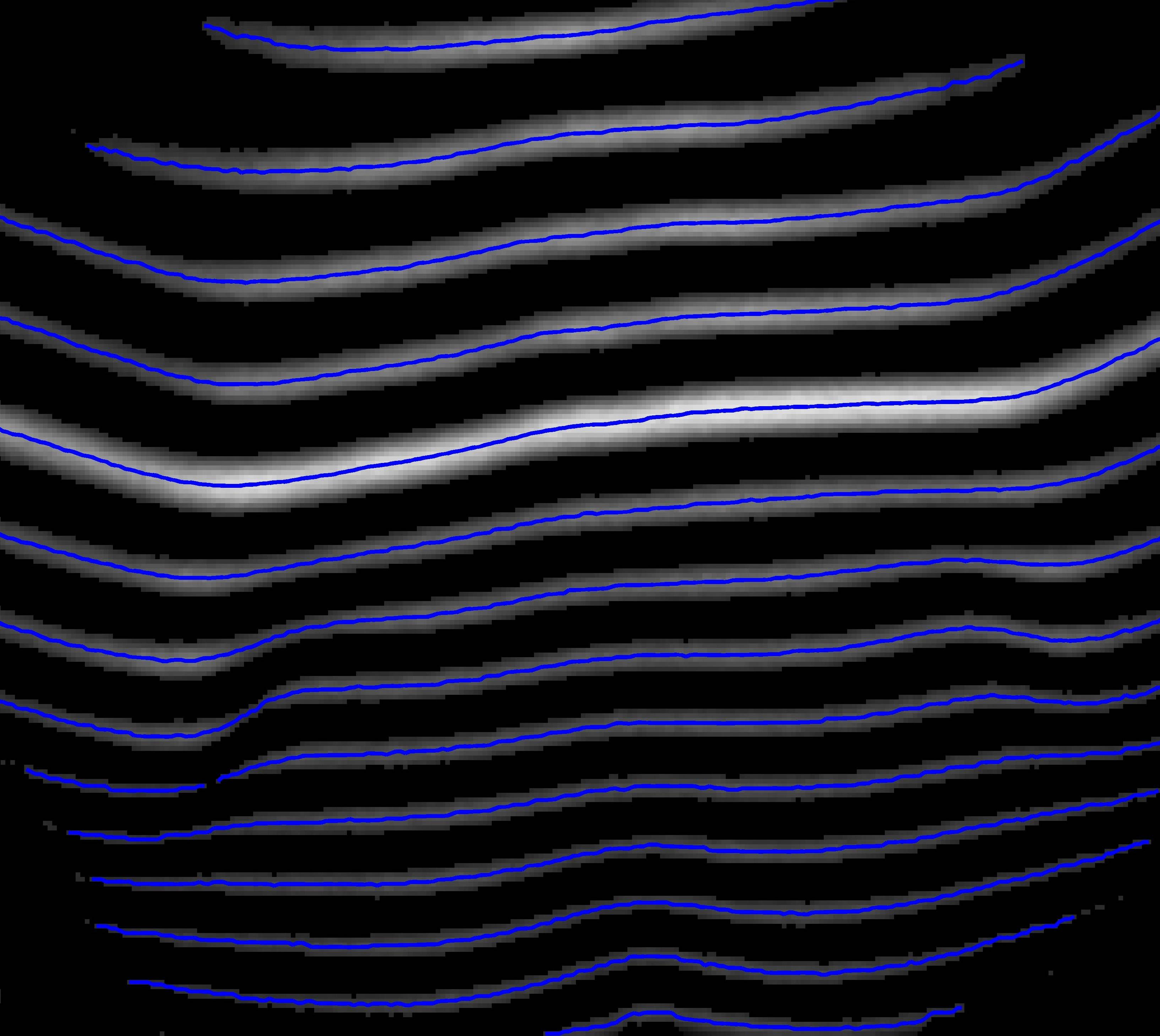
These are the curves that are found by finding the weighted average per column:

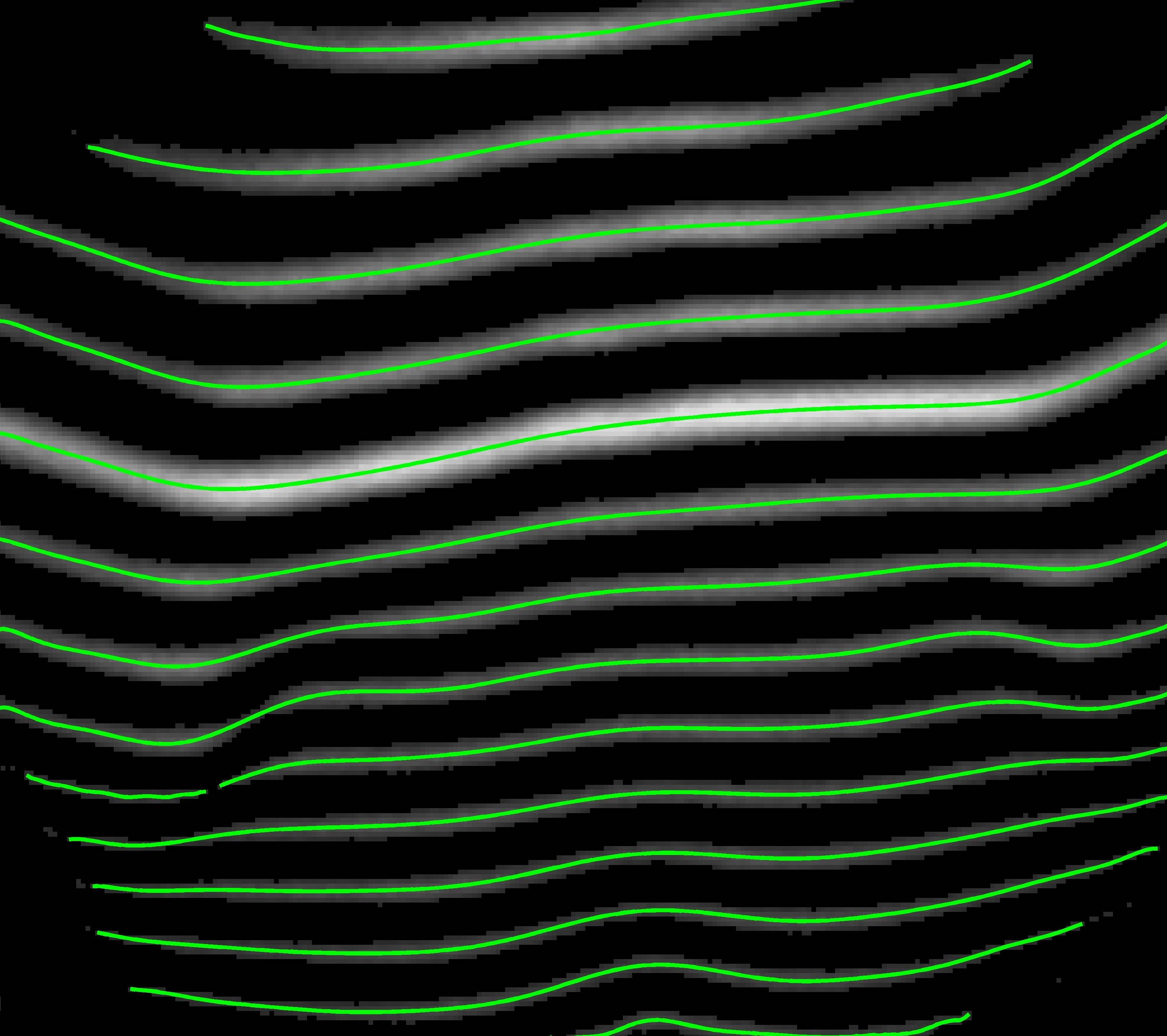
These are the curves after fitting a polynomial:

Here is the code:

function Zebra()
    im = imread('https://i.sstatic.net/m0sy7.png');
    im = uint8(mean(im,3));

    th = 40;
    imBinary = im>th;
    imBinary = imclose(imBinary,strel('disk',2));
    % figure;imshow(imBinary);
    labels = logical(imBinary);
    props =regionprops(labels,im,'Image','Area','BoundingBox');

    figure(1);imshow(im .* uint8(imBinary));
    figure(2);imshow(im .* uint8(imBinary));

    for i=1:numel(props)
        %Ignore small ones
        if props(i).Area < 10
            continue
        end
        %Find weighted centroids
        boundingBox = props(i).BoundingBox;
        ul = boundingBox(1:2)+0.5;
        wh = boundingBox(3:4);
        clipped = im( ul(2): (ul(2)+wh(2)-1), ul(1): (ul(1)+wh(1)-1) );
        imClip = double(props(i).Image) .* double(clipped);
        rows = transpose( 1:size(imClip,1) );
        %Weighted calculation
        weightedRows  = sum(bsxfun(@times, imClip, rows),1) ./ sum(imClip,1);
        %Calculate x,y
        x = ( 1:numel(weightedRows) ) + ul(1) - 1;
        y = ( weightedRows ) + ul(2) - 1;
        figure(1);
        hold on;plot(x,y,'b','LineWidth',2);
        try %#ok<TRYNC>
            figure(2);
            [xo,yo] = FitCurveByPolynom(x,y);
            hold on;plot(xo,yo,'g','LineWidth',2);
        end
        linkaxes( cell2mat(get(get(0,'Children'),'Children')) )
    end        
end

function [xo,yo] = FitCurveByPolynom(x,y)
   p = polyfit(x,y,15); 
   yo = polyval(p,x);
   xo = x;
end

Answer 2

I wouldn't use the RGB image. Color images are typically made by putting a "Bayer Filter" on the camera sensor, which usually reduces the resolution you can achieve.

If you use the grayscale image, I think the steps you described (binarize "zebra" image, find midline) are a good start. As a final step, I would

• Take each point in the midline you found
• take the grayvalues of the pixels in the "zebra" line above and below
• fit a parabola to these grayvalues using least mean squares
• the apex of this parabola is an improved estimate of the midline position

Answer 3

Here is yet an alternative solution to your problem by modelling your question as a 'path optimization problem'. Though it is more complicated than the simple binarization-and-then-curvefitting solution, it is more robust in practice.

From the very high level, we should consider this image as a graph, where

1. each image pixel is a node on this graph

2. each node is connected to some other nodes, known as neighbours, and this connection definition is often referred as to the topology of this graph.

3. each node has a weight (feature, cost, energy, or whatever you want to call it ), reflecting the likelihood that this node is in an optimal central-line we are looking for.

As long as we can model this likelihood, then your problem of finding 'the centerlines of the fringes' becomes to the problem to find local optimal paths on the graph, which can be effectively solved by dynamic programming, e.g. Viterbi algorithm.

Here are some pros of adopting this approach:

1. all your results will be continuous ( unlike the threshold method that might break one center line into pieces )

2. a lot of freedoms to construct such a graph, you can select different features, and graph topology.

3. your results are optimal in the sense of path optimizations

4. your solution will be more robust against noise, because as long as noise is equally distributed among all pixels, those optimal paths remain stable.

Here is a short demonstration of the above idea. Since I donot use any prior knowledge to specify what are possible starting and ending nodes, I simply decode w.r.t every possible starting node.

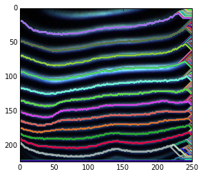
For the fuzzy endings, it is caused by the fact that we are looking for optimal paths for every possible ending nodes. As a result, though for some nodes located in dark areas, the highlighted path is still its local optimal one.

For the fuzzy path, you could either smooth it after you find it or use some smoothed features instead of raw intensity.

It is possible to restore partial paths by changing starting and ending nodes.

It will not be difficult to prune these undesired local optimal paths. Because we have the likelihoods of all paths after viterbi decoding, and you may use various prior knowledge ( e.g. we see it is true that we only need one optimal path for those sharing the same source. )

For more details, you may refer to the paper.

 Wu, Y.; Zha, S.; Cao, H.; Liu, D., & Natarajan, P.  (2014, February). A Markov Chain Line Segmentation Method for Text Recognition. In IS&T/SPIE 26th Annual Symposium on Electronic Imaging (DRR), pp. 90210C-90210C.

Here is a short piece of python code using to make the above graph.

import cv2
import numpy as np
from matplotlib import pyplot
# define your image path
image_path = ;
# read in an image
img = cv2.imread( image_path, 0 );
rgb = cv2.imread( image_path, -1 );

# some feature to reflect how likely a node is in an optimal path
img = cv2.equalizeHist( img ); # equalization
img = img - img.mean(); # substract DC
img_pmax = img.max(); # get brightest intensity
img_nmin = img.min(); # get darkest intensity
# express our preknowledge
img[ img > 0 ] *= +1.0  / img_pmax; 
img[ img = 1 :
    prev_idx = vt_path[ -1 ].astype('int');
    vt_path.append( path_buffer[ prev_idx, time ] );
    time -= 1;
vt_path.reverse();    
vt_path = np.asarray( vt_path ).T;

# plot found optimal paths for every 7 of them
pyplot.imshow( rgb, 'jet' ),
for row in range( 0, h, 7 ) :
    pyplot.hold(True), pyplot.plot( vt_path[row,:], c=np.random.rand(3,1), lw = 2 );
pyplot.xlim( ( 0, w ) );
pyplot.ylim( ( h, 0 ) );

Answer 4

Thought I should post my answer as it is bit different from other approaches. I tried this in Matlab.

• sum all channels and create an image, so all channels are weighted equally
• perform morphological closing and Gaussian filtering on this image
• for each column of the resulting image, find the local maxima and construct an image
• find the connected components of this image

One disadvantage I see here is that this approach will not perform well for some orientations of the stripes. In that case we have to correct its orientation and apply this procedure.

Here's the Matlab code:

im = imread('m0sy7.png');
imsum = sum(im, 3); % sum all channels
h = fspecial('gaussian', 3);
im2 = imclose(imsum, ones(3)); % close
im2 = imfilter(im2, h); % smooth
% for each column, find regional max
mx = zeros(size(im2));
for c = 1:size(im2, 2)
    mx(:, c) = imregionalmax(im2(:, c));
end
% find connected components
ccomp = bwlabel(mx);

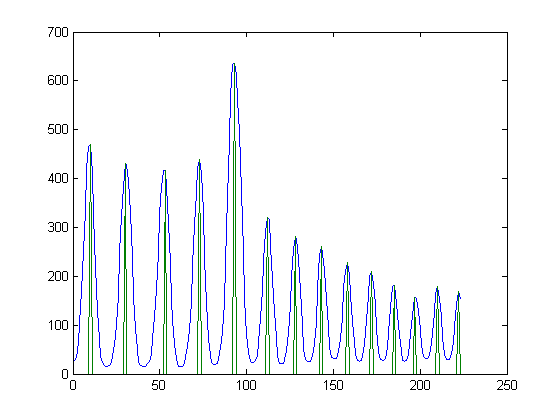
For example, if you take the mid column of the image, its profile should look like this: (in blue is the profile. in green are the local maxima)

And the image containing the local maxima for all columns looks like this:

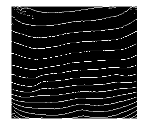
Here are the connected components (though some stripes are broken, most of them get a continuous region):