Discrete approximation to Gaussian filter

Question

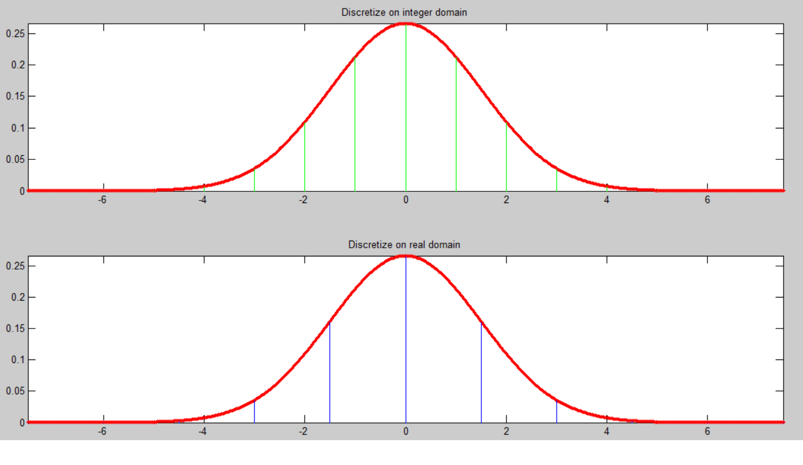
One method of producing a discrete approximation kernel to a Gaussian filter of variance $\sigma^2$ is to assume a cutoff of $5\sigma$. This seems to suggest the following procedure:

1. Create a uniform grid $\mathbb{x}$ of size $11(=2*5+1)$ between $[-5\sigma,5\sigma]$
2. Evaluate $\mathcal{N}(\mathbb{x};0,\sigma)$ and obtain the discrete approximation.

The blue lines in the second plot below depict the discretized values(for $\sigma=1.5$). In this case, the result is not a proper filter kernel since the sum of values is not $1$.

But MATLAB's fspecial does things a bit differently. For the call fspecial('gaussian',[1 11],sigma)

1. Create a uniform grid $\mathbb{x}$ of size $11(=2*5+1)$ between $[-5,5]$
2. Compute $\mathbb{x}'= e^{\frac{-\mathbb{x}^2}{2\sigma^2}}$
3. Normalize $\mathbb{x}'$ so that it sums to $1$

The green lines in the first plot below the values as computed by MATLAB's fspecial(for $\sigma=1.5$).

What is the difference between both methods ?

Answer 1

The difference between the two should be slight but the MATLAB one has the property that it preserves the signal energy content. That is a property that you expect to have when using a Gaussian filter.

Answer 2

The first method involves computation of the Gaussian function including its normalization factor. The normalization factor is relevant for the full distribution. In fact, evaluating it at discrete points is not correct since it is meant to be used for a continuous distribution. However, even if we omit the normalization factor from the function, we could still use the uniformly discretized $[-5\sigma,5\sigma]$ to compute the filter. In fact, the first method has the nice property that filter values fall at intervals of $\sigma$.

Most likely, the second method(MATLAB's) is used since we are guaranteed to have uniform discretization (stepping in integer increments) unlike the first method.

However, while plotting, we do need to use the normalization factor to ensure the vertical lines(green,blue lines in plots shown) line up nicely.