Here are some options to consider:
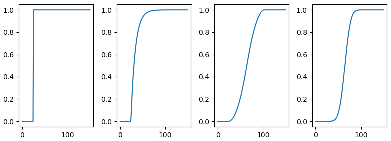
The first plot is the input step.
The second plot is the result with the exponential moving average filter as given by the OP.
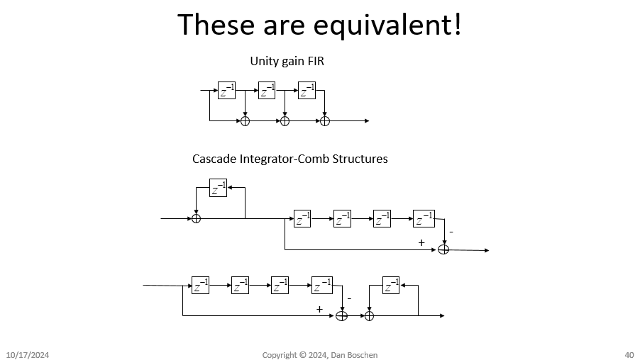
The third plot is the result of using two moving average filters in cascade. (A moving average filter is an FIR filter with unity gain coefficients and then scaled by the sum of the coefficients, so passing through this filter twice or convolving the coefficients to be a single filter). You can also achieve a moving average filter by cascading an accumulator with a difference filter (as a CIC) as follows:
I used two moving average filters each over 40 samples for the resulting plot I gave above so the difference if done as a CIC would be $1-z^{-40}$.
The fourth plot is the result of using a Gaussian Filter. This is the result of a FIR filter with coefficients given by a Gaussian. You can also get that by repeatably passing the signal through a two tap FIR filter with unity gain coefficients scaled by 1/2 ([0.5, 0.5]), which will approach a Gaussian as given by the Central Limit Theorem.
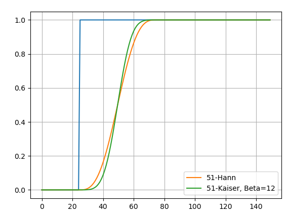
Another option is to use a standard window as the coefficients for an FIR filter (any of the windows that are available in Matlab, Octave, or scipy.signal would be suitable creating such transitions, resulting in a symmetric weighted moving average which is what is needed).
Below is a demonstration with the Hann window and Kaiser window. The transition duration is set by the length of the window used. I like Kaiser as you can adjust the taper directly to match that of most of the other windows just by changing $\beta$.


