Return to Revisions

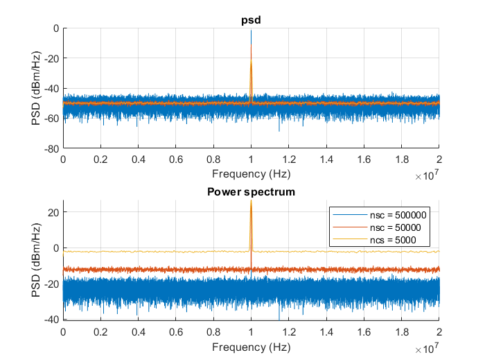
The PSD is appropriate if one is interested in consistent noise power levels. If you want consistent signal power levels, you should compute the power spectrum, which uses a different scaling factor.

Denote by $|X|^2$ the frequency averaged Squared Magnitude Spectrum and $w$ the window applied.

• The PSD is: $$\frac{2|X|^2}{f_s \times S_2} \quad S_2 = \sum_{i = 0}^{N - 1} w_i^2$$
• The Power Spectrum is: $$\frac{2|X|^2}{S_1^2} \quad S_1 = \sum_{i = 0}^{N - 1} w_i$$

Add a little noise to your pure tone, and notice how the noise power stays the same but signal power fluctuates when you change nsc with the PSD, and how the opposite is true when using the Power Spectrum:

To replicate:

close all
fs = 20e7;
sine = dsp.SineWave('Amplitude',1,'Frequency',10e6,'SampleRate',fs,'SamplesPerFrame',1000000);
y = sine();
y = y+ randn(length(y),1);

figure(1)
subplot 211
title('psd')
hold on
subplot 212
title('Power spectrum')
hold on
for method = {'psd', 'power'}
    for nsc = [500000, 50000, 5000]
        nov = floor(nsc/2);
        nff = max(256,2^nextpow2(nsc));

        [pxx, f] = pwelch(y,hann(nsc),nov,nff,fs, string(method));
        pxx = 10*log10(pxx) + 30; % also convert to dBm
        
        
        if strcmp(string(method), "psd")
            subplot 211
        else
            subplot 212
        end
        plot(f, pxx);
        grid on;
        xlim([0 20e6]);
        xlabel("Frequency (Hz)");
        ylabel("PSD (dBm/Hz)");
    end
end
legend('nsc = 500000', 'nsc = 50000', 'nsc = 5000')