Excerpted from Jae S.Lim 2D signal and image processing ch.1, as an example of $2$-D circularly symmetric lowpass filter with a cutoff frequency of $\omega_c$ radians per sample, whose impulse response is given by: $$h[n_1,n_2] = \frac{\omega_c}{2\pi \sqrt{n_1^2 + n_2^2} } J_1 \big( \omega_c \sqrt{n_1^2 + n_2^2} \big) $$
where $J_1$ is the Bessel function of the first kind and the first order...
Interested readers may consult the book for a derivation which is not untitive but nevertheless tractable; familiarity with Bessel functions is required but also provided as is.
Olli's edits: At $n_1 = n_2 = 0$ the limiting value must be used:
$$h[0, 0] = \frac{\omega_c^2}{4\pi}$$
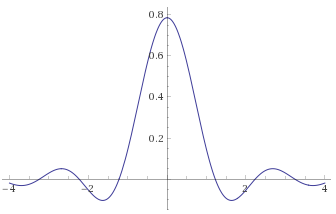
A slice through the middle of $h[n_1,n_2]$ with $\omega_c = \pi$:
Python source for 2-d filter kernel (you may want to apply a 2-d window function):
import scipy
inport numpy as np

def circularLowpassKernel(omega_c, N):  # omega = cutoff frequency in radians (pi is max), N = horizontal size of the kernel, also its vertical size, must be odd.
  kernel = np.fromfunction(lambda x, y: omega_c*scipy.special.j1(omega_c*np.sqrt((x - (N - 1)/2)**2 + (y - (N - 1)/2)**2))/(2*np.pi*np.sqrt((x - (N - 1)/2)**2 + (y - (N - 1)/2)**2)), [N, N])
  kernel[(N - 1)//2, (N - 1)//2] = omega_c**2/(4*np.pi)
  return kernel
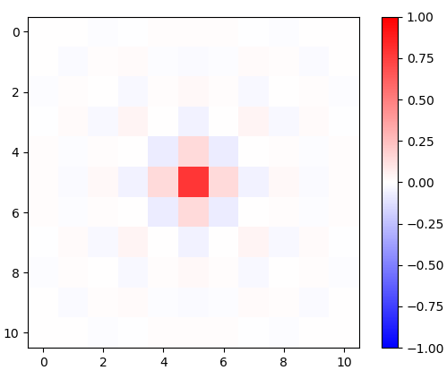
Example with $\omega_c = \pi$:
import matplotlib.pyplot as plt

kernelN = 11  # Horizontal size of the kernel, also its vertical size. Must be odd.
omega_c = np.pi  # Cutoff frequency in radians <= pi
kernel = circularLowpassKernel(np.pi, kernelN)
plt.imshow(kernel, vmin=-1, vmax=1, cmap='bwr')
plt.colorbar()
plt.show()


