I am playing around with a 3 axis magnetometer to gather real world readings. I am trying to see how accurately I can measure the 50Hz component of an electric field around a mains wire. Now, obviously, if there are 2 conductors, one going up and the other going down, they will cancel each other out (mostly), so I am measuring with a single conductor and I can definitely see some significant magnetic fields. I am however struggling to settle on a good DSP algorithm to measure the 50Hz component.
Constaints
- I can measure at either 155 Hz or 300 Hz with the equipment I have.
- It is advantageous power-wise that I keep the measurement window fairly short (i.e. half a second or less if possible).
- I have a reasonable but still limited amount of processing power on my little ESP32 that I'm using to play with.
Progress
I can measure at either frequency and the results look sensible. If I use 300 Hz to demonstrate. Let me drop in 2 data sets as csv - one when there is very little field, and one when there is heaps! Can't seem to attach as csv. So sorry, but will paste in at the end.
Embedded Code
I'm working on 2 things. First in embedded C, I've got this going on:
- measure x, y & z
- calculate average x, y & z
- remove dc offset
- create a magnitude variable like this:
obs.mag[i] = sqrt(pow(obs.data[i].mx, 2) + pow(obs.data[i].my, 2) + pow(obs.data[i].mz, 2));
- bandpass 5th order iir at 50 Hz with Q = 10.
- zero fill imaginary part and fft
- try to get power as follows:
for (int i = 0 ; i < N / 2 ; i++) { obs.fft_complex[i] = 10 * log10f((obs.fft_complex[i * 2 + 0] * obs.fft_complex[i * 2 + 0] + obs.fft_complex[i * 2 + 1] * obs.fft_complex[i * 2 + 1]) / N); }
- Grab a measure of the power at 50Hz:
float linear_power_50hz = pow(10, obs.fft_complex[BIN_50HZ] / 10);
R Studio
And secondly in R Studio, I'm having a play there too, to see if my readings make sense. My R code is as follows:
    # Read the CSV file
  data <- read.csv("obs/biggie_field.csv")

  # Define sampling frequency and create a time vector
  fs <- 300  # Sampling frequency in Hz
  time <- seq(0, (nrow(data)-1)/fs, by = 1/fs)

  # Plot original time domain signal for mx component
  ggplot(data.frame(time, mx = data$mx), aes(x = time, y = mx)) +
    geom_line() +
    labs(title = "Original Time Domain Signal (mx)", x = "Time (s)", y = "Magnetic Field (T)")

  # Design a 5th-order Butterworth bandpass filter
  low_cut <- 45 / (fs/2)  # Lower cutoff frequency normalized to Nyquist frequency
  high_cut <- 55 / (fs/2) # Upper cutoff frequency normalized to Nyquist frequency
  iir_filter <- butter(5, c(low_cut, high_cut), type = "pass")

  # Apply the filter to mx, my, mz components
  filtered_mx <- filtfilt(iir_filter, data$mx)
  filtered_my <- filtfilt(iir_filter, data$my)
  filtered_mz <- filtfilt(iir_filter, data$mz)

  # Plot filtered time domain signal for mx component
  ggplot(data.frame(time, filtered_mx), aes(x = time, y = filtered_mx)) +
    geom_line() +
    labs(title = "Filtered Time Domain Signal (mx)", x = "Time (s)", y = "Magnetic Field (T)")

  # Compute FFT for the filtered signal
  fft_result_filtered <- fft(filtered_mx)
  power_filtered <- Mod(fft_result_filtered)^2 / length(filtered_mx)

  # Plot power spectrum after filtering
  plot_data_filtered <- data.frame(freq = (0:(length(filtered_mx)-1)) * (fs/length(filtered_mx)),
                                   power = power_filtered)
  ggplot(plot_data_filtered, aes(x = freq, y = power)) +
    geom_line() +
    xlim(0, 80) +
    labs(title = "Power Spectrum After Filtering", x = "Frequency (Hz)", y = "Power")

  # Output the power at 50 Hz after filtering
  closest_idx_filtered <- which.min(abs(plot_data_filtered$freq - 50))
  power_at_50Hz_filtered <- plot_data_filtered$power[closest_idx_filtered]

  power_at_50Hz_filtered
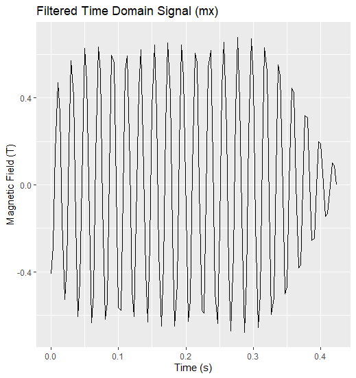
And I get some pretty convincing results. The time domain plot looks liek this:
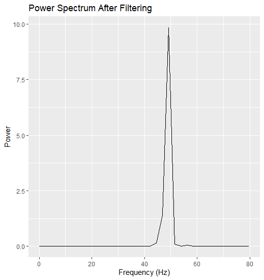
And the final power plot is like this:
Help
My goal is to output a relative metric of power. I.e. so long as the output for 1000 W is ten times bigger than that for 100 W, I'm happy.
Is my R plan sound? If so, I'll try to replicate in embedded code.
BIGGIE
------
mx,my,mz
-1.572180,0.572764,0.383986
-0.927528,-0.102864,-0.229106
-0.473407,-0.267095,-0.424898
-0.135009,-0.415546,-0.594389
-0.586791,0.296318,0.053185
-1.278784,0.490941,0.217417
-1.724138,0.583285,0.338983
-1.315020,-0.009936,-0.225015
-0.572764,-0.282876,-0.362361
-0.132671,-0.507306,-0.507890
-0.303916,0.078317,0.060199
-1.140853,0.481005,0.210403
-1.493863,0.783168,0.344828
-1.582700,0.381648,-0.223846
-0.686733,-0.221508,-0.383986
-0.431327,-0.623027,-0.537113
-0.214494,-0.317358,0.031560
-1.068966,0.392753,0.222677
-1.292811,0.781414,0.363530
-1.531268,0.620105,-0.167738
-0.708358,-0.130333,-0.386908
-0.513150,-0.471654,-0.565167
-0.244886,-0.471654,-0.075979
-1.067797,0.313267,0.219170
-1.286967,0.573933,0.413209
-1.533606,0.735827,0.018118
-0.697253,-0.066043,-0.375804
-0.498539,-0.259497,-0.619521
-0.321449,-0.451198,-0.268264
-1.122735,0.259497,0.170076
-1.285213,0.453536,0.443016
-1.428989,0.649328,0.199883
-0.678551,-0.069550,-0.305085
-0.462303,-0.226768,-0.569842
-0.300409,-0.457627,-0.506721
-1.082992,0.281707,0.100526
-1.334892,0.450029,0.352425
-1.472823,0.596143,0.351257
-0.793688,-0.100526,-0.247224
-0.459965,-0.257744,-0.454705
-0.182934,-0.390999,-0.538866
-0.793688,0.288136,0.060199
-1.305085,0.488019,0.232028
-1.701344,0.606663,0.397428
-1.285798,-0.057861,-0.219170
-0.539451,-0.288136,-0.363530
-0.095850,-0.483928,-0.542373
-0.324956,0.152542,0.054939
-1.192285,0.494448,0.193454
-1.617183,0.731736,0.340736
-1.551140,0.202805,-0.237288
-0.644068,-0.254237,-0.378141
-0.295149,-0.580362,-0.538866
-0.193454,-0.173583,0.049679
-1.084161,0.436587,0.207481
-1.364699,0.825248,0.353594
-1.593805,0.556984,-0.198714
-0.706020,-0.160140,-0.395675
-0.502630,-0.546464,-0.555815
-0.250146,-0.440678,-0.030976
-1.057861,0.313267,0.224430
-1.276447,0.613092,0.399766
-1.484512,0.684395,-0.047341
-0.682057,-0.079486,-0.378726
-0.507306,-0.316189,-0.614845
-0.241964,-0.542373,-0.265926
-1.102864,0.251899,0.188194
-1.276447,0.455289,0.443600
-1.450614,0.674459,0.167738
-0.658095,-0.059030,-0.323203
-0.470485,-0.231444,-0.588545
-0.327878,-0.436587,-0.426651
-1.102864,0.265342,0.137347
-1.323787,0.436587,0.389246
-1.459381,0.655172,0.382233
-0.715956,-0.095850,-0.260666
-0.451783,-0.252484,-0.490941
-0.212157,-0.417884,-0.550555
-0.907072,0.306254,0.065459
-1.324372,0.469901,0.279369
-1.642314,0.591467,0.373466
-1.057861,-0.084746,-0.222677
-0.498539,-0.289889,-0.388077
-0.064290,-0.430742,-0.554062
-0.416715,0.233781,0.068381
-1.225015,0.494448,0.205728
-1.667446,0.663939,0.376388
-1.509643,0.124489,-0.218001
-0.623027,-0.261251,-0.369375
-0.244302,-0.578025,-0.510228
-0.216832,-0.081239,0.075395
-1.103448,0.448276,0.223261
-1.393922,0.818819,0.350672
-1.556400,0.466978,-0.198130
-0.704851,-0.189363,-0.371712
-0.481005,-0.595558,-0.544126
-0.174167,-0.447107,-0.008182
-1.064290,0.351841,0.237288
-1.276447,0.691409,0.393337
-1.518995,0.690824,-0.085915
-0.713033,-0.094681,-0.375219
-0.500292,-0.355932,-0.590298
-0.267680,-0.488019,-0.161894
-1.085915,0.270602,0.212157
-1.279369,0.469316,0.455289
-1.512566,0.731736,0.156049
-0.664524,-0.045587,-0.326125
-0.481590,-0.235535,-0.599065
-0.288720,-0.471654,-0.390415
-1.122735,0.269433,0.142022
-1.329632,0.434833,0.410286
-1.430158,0.609001,0.303916
-0.693746,-0.077732,-0.268849
-0.445938,-0.233781,-0.511397
-0.246055,-0.410871,-0.552309
-0.947399,0.310345,0.077732
-1.338983,0.465225,0.284629
-1.596143,0.592636,0.389830
-0.995909,-0.097019,-0.224430
-0.481590,-0.263004,-0.405026
-0.093513,-0.399182,-0.534775
-0.552893,0.272355,0.060199
-1.258913,0.488019,0.197545
-1.704851,0.631794,0.352425
-1.441262,0.043250,-0.227937
-0.600234,-0.275862,-0.368790
-0.189363,-0.535359,-0.538866
-0.182350,-0.046172,0.064290

TINY
----
mx,my,mz
-0.945061,0.317358,-0.463472
-0.952659,0.312098,-0.462887
-0.942724,0.319112,-0.460549
-0.942139,0.317943,-0.454120
-0.940970,0.320281,-0.464641
-0.946230,0.319112,-0.459380
-0.944477,0.320281,-0.464056
-0.943892,0.317943,-0.458212
-0.941555,0.320281,-0.461718
-0.946230,0.318527,-0.463472
-0.946815,0.313852,-0.465809
-0.943308,0.316774,-0.463472
-0.939801,0.319112,-0.462887
-0.942724,0.321449,-0.470485
-0.945646,0.317943,-0.457627
-0.940970,0.320281,-0.461134
-0.941555,0.315605,-0.462303
-0.943892,0.318527,-0.458796
-0.940386,0.322034,-0.465225
-0.945646,0.316189,-0.465809
-0.938632,0.311514,-0.466394
-0.947399,0.319696,-0.465809
-0.939801,0.313267,-0.456458
-0.941555,0.316189,-0.465225
-0.945061,0.313267,-0.466978
-0.940970,0.314436,-0.458796
-0.945646,0.310929,-0.462887
-0.945646,0.316189,-0.461718
-0.943892,0.312098,-0.459380
-0.937463,0.314436,-0.457043
-0.942139,0.312683,-0.465225
-0.945061,0.312683,-0.455289
-0.943308,0.311514,-0.455289
-0.947399,0.317358,-0.456458
-0.943308,0.312683,-0.447107
-0.943308,0.312098,-0.456458
-0.942139,0.313852,-0.454705
-0.945646,0.312683,-0.458796
-0.946230,0.315020,-0.459965
-0.943892,0.312683,-0.462887
-0.943892,0.315020,-0.457627
-0.939801,0.312098,-0.457627
-0.949737,0.319696,-0.452367
-0.943892,0.313852,-0.461718
-0.943892,0.313267,-0.454705
-0.945061,0.312683,-0.455289
-0.949737,0.313267,-0.454705
-0.949153,0.313852,-0.454705
-0.949737,0.314436,-0.457043
-0.946815,0.311514,-0.455874
-0.947399,0.311514,-0.452951
-0.946815,0.310929,-0.455289
-0.948568,0.314436,-0.451783
-0.944477,0.307423,-0.454120
-0.942139,0.313852,-0.457627
-0.946815,0.308591,-0.457043
-0.943892,0.309176,-0.457043
-0.943892,0.307423,-0.452367
-0.943308,0.310929,-0.455289
-0.946230,0.309176,-0.463472
-0.945646,0.316189,-0.459965
-0.942139,0.312098,-0.458796
-0.942139,0.310929,-0.461718
-0.945646,0.310345,-0.460549
-0.943308,0.314436,-0.460549
-0.946815,0.312098,-0.456458
-0.950321,0.307423,-0.455289
-0.946230,0.311514,-0.455874
-0.950906,0.312683,-0.454120
-0.945061,0.308591,-0.452951
-0.949153,0.316189,-0.454705
-0.946230,0.314436,-0.451783
-0.948568,0.313267,-0.448860
-0.946815,0.311514,-0.454120
-0.946230,0.314436,-0.457627
-0.942724,0.309760,-0.449445
-0.944477,0.317358,-0.454120
-0.945646,0.316189,-0.451198
-0.946815,0.312098,-0.455289
-0.949737,0.309176,-0.455874
-0.939801,0.314436,-0.453536
-0.952659,0.315020,-0.454705
-0.946815,0.312683,-0.464641
-0.945061,0.312683,-0.458212
-0.944477,0.308591,-0.459380
-0.947399,0.312683,-0.462303
-0.949153,0.316774,-0.457043
-0.942139,0.313267,-0.458212
-0.946815,0.310929,-0.460549
-0.943892,0.310345,-0.457043
-0.940386,0.312098,-0.458796
-0.943308,0.313267,-0.464641
-0.948568,0.315605,-0.466978
-0.943892,0.313267,-0.461134
-0.949153,0.310345,-0.464056
-0.944477,0.310929,-0.462303
-0.943308,0.312683,-0.452951
-0.940970,0.317943,-0.452951
-0.946815,0.317358,-0.459965
-0.947984,0.319696,-0.454705
-0.949153,0.317358,-0.463472
-0.948568,0.318527,-0.455874
-0.946815,0.312098,-0.458796
-0.947984,0.317358,-0.458212
-0.943308,0.313852,-0.457627
-0.945061,0.308591,-0.459965
-0.947984,0.314436,-0.465809
-0.949153,0.309760,-0.454120
-0.945646,0.313267,-0.458796
-0.943308,0.313267,-0.455874
-0.947984,0.309760,-0.454705
-0.946230,0.314436,-0.458796
-0.940970,0.312098,-0.462303
-0.945061,0.306838,-0.462887
-0.947399,0.315605,-0.457043
-0.943892,0.310929,-0.457627
-0.942139,0.308591,-0.455874
-0.947984,0.307423,-0.462303
-0.946230,0.309176,-0.458212
-0.947399,0.308007,-0.461718
-0.943892,0.311514,-0.451783
-0.945061,0.310929,-0.462887
-0.940970,0.317358,-0.458796
-0.943892,0.315020,-0.457627
-0.947984,0.315605,-0.455874
-0.942724,0.318527,-0.457043
-0.943308,0.311514,-0.464056
-0.943892,0.311514,-0.461718


