Interpretation of a non-canonical Allan Variance plot

Question

I am currently working on characterizing the noise sources of a Global Navigation Satellite System (GNSS) sensor using an Allan Variance plot, which is commonly employed to analyze frequency stability in atomic clocks, but has since been extended to other applications such as Inertial Measurement Units (IMUs) and sensors.

A typical (modified) Allan Deviation plot exhibits a distinctive "bowl" shape where different noise contributors are distinctly represented (see Wikipedia and Example).

In order to characterize the diverse noise sources affecting each component of the GNSS sensor, I collected data at a fixed location for five consecutive days with samples recorded every 0.05 seconds (20 Hz), under two separate configurations:

• Antenna facing upward
• Antenna facing sideways

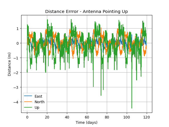
Below is an extract from the obtained data (antenna up):

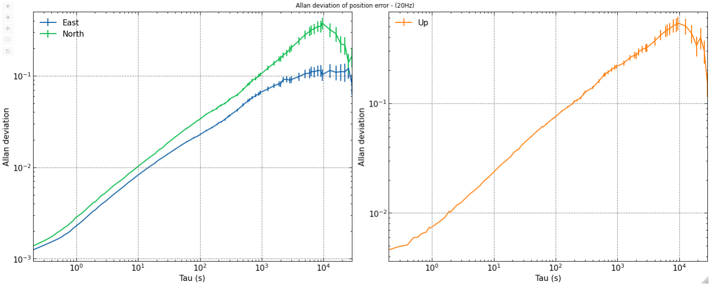
Assuming precise knowledge of the receiver's position, I computed the errors and plotted their respective Allan deviations for both configurations, depicted as follows:

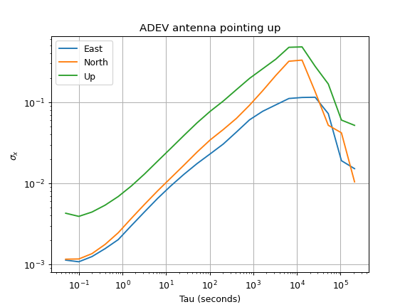
For the antenna facing up, I get the following Allan curve (in meters [m]):

For the antenna facing sideways, I get the following curve (in meters [m]):

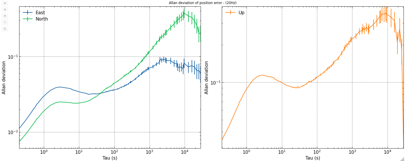
As observed, these Allan deviations hint towards a dominant presence of random walk noise, which contradicts expectations of boundedness. Specifically, I expect a GNSS estimate to fluctuate around the true value, due to factors like atmospheric conditions, satellite constellation geometry, clock biases, etc.

Thus, the assumption about noise interpretation must be incorrect as random walk is by definition unbounded. I would appreciate suggestions for accurately interpreting these results.

Additionally, I provide Fast Fourier Transform (FFT) representations of the errors, here and here.

These FFT outputs seem consistent with the random walk conjecture when compared against canonical noises examples (see this document, top of page 6 for an example of different noises FFT).

My analysis of the noise in the signal based on the Allan variance curves is therefore wrong. Would you have a suggestion for reading these curves correctly?

Any help is greatly appreciated. Thank you very much.

[EDIT] - The Allan Variance function used to perform the above analysis is the below. It is derived from the paper Bridging the gap between sensor noise modeling and sensor characterization:

def allanDeviation2(signal: np.ndarray, dt: float):
    """
    Implementation of allan deviation computation from the paper
    https://www.sciencedirect.com/science/article/abs/pii/S026322411730578X?via%3Dihub
    """

    # Size tau vector
    N = len(signal)
    orderMax = int(np.log10(N * dt) + 1) - 2  # Number of digits in final time (minus two for some reason...)
    order = int(np.log10(dt))

    # Generate tau vector
    base = np.array([2, 3, 4, 5, 6, 7, 8, 9])
    tauVec = np.array([])

    while order < orderMax:
        tauVec = np.concatenate((tauVec, 10 ** order * base))
        order += 0.5

    tauVec = np.sort(tauVec)
    allanDev = np.zeros(len(tauVec))

    # For each tau, calculate the Allan Deviation
    for i, tau in enumerate(tauVec):
        t = round(tau / dt)  # Number of measurements in this tau bin
        nDivisions = int(N // t)

        # Calculate the average for each block of data
        avg = np.average(signal[: nDivisions * t].reshape(-1, t), axis=1)  # Very fast thanks to Jon

        # Calculate the Allan Variance on the difference of two successive averages
        diff = np.diff(avg)
        allanDev[i] = np.sqrt(1 / 2 * np.average(diff ** 2))

    error = allanDev / np.sqrt(N * dt / tauVec + 1)

    return tauVec, allanDev, error

You can find the test of this function to different noise sources in this pdf document.

[EDIT 2]: You can find the dataset here (numpy and CSV format). Order is ENU.

Answer 1

The analysis appears to be correct. I reviewed the OP's code and did not see a fault with the process used to compute ADEV on the OP's dataset. Further, I downloaded the OP's code and cross-validated using the trusted Python package "allantools" for computing ADEV (using my preference of "Overlap ADEV" which has a tighter confidence interval to the same "underlying truth" for the same dataset due to overlapping the data in the computation).

The result, out to 10,000 seconds is indeed consistent with a Random Walk process. When we look at the data in the time domain, unlike a true Random Walk process, the data appears to be stationary in the long term. We also see a long term convergence behavior in the ADEV when we go past 100,000 seconds (although I typically don't trust results in the last decade of an ADEV plot due to the substantially less number of samples used to compute the computation there-- however I suspect in seeing the time domain data and understanding the application that in the very long term, the ADEV will go down at a $1/\tau$ rate consistent with what we get with GPS timing as a white phase noise process. The ADEV above does seem to show this $1\tau$ behavior after 10,000 seconds.)

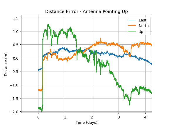
So in the short term the data is indeed characteristic of a random walk; this is intuitively clear if we zoom in on the time domain data and consider only a short duration:

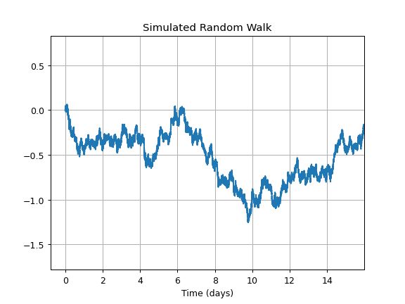
The above is very much what samples of a random walk process would look like. Below shows a simulated random walk by accumulating samples of AWGN (Additive White Gaussian Noise) where it is hard to tell the difference statistically between our simulated and actual values above (this is because, over this short duration, there is no difference statistically!) [this was with an accumulator, implementing random walk over the full duration of the samples; if we were to implement a "leaky integrator", that would closely model the OP's process with a longer term convergence]:

This process, that is random walk in the nearer term, but in the longer term does converge back to the mean and is ultimately stationary, is known as a Ornstein_Uhlenbeck process. We can get further insight by evaluating the OP's data in the frequency domain with a power spectral density using the Welch algorithm as shown below:

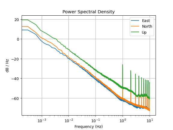
Here we see the 20 dB/decade roll-off consistent with a random walk process. If we were to continue to take data in the longer term, what we would expect to see is the low frequency end of the power spectral density level out as we approach DC, as opposed to a true random walk process that would continue to grow without bound. ADEV as a simple explanation is the standard deviation of a signal after bandpass filtering, and the center frequency of that filter is the reciprocal of the averaging time $\tau$ shown on the horizontal axis of the ADEV result. Thus for the process plotted in the PSD above, we see how as the averaging time is increased the power after the effective bandpass filter of the ADEV computation could increase (given the center frequency of that filtering decreases).

Note the 1 Hz tones and higher harmonics that are also present in the signal. A sinusoidal interference has a tell-tale shape in ADEV where it peaks at roughly half the frequency and has a first null at the frequency and nulls at higher harmonics of the frequency, with the peaks going down at $1/\tau$. We see absolutely no sign of this in the ADEV results, which means the additive noise due to the sinusoidal interference is buried in the random walk noise that dominates at these time offsets.