1
$\begingroup$

I am working on a radar signal processing project using MATLAB. I am required to simulate range doppler maps for Linear Frequency-Modulation (LFM) targets (non-fluctuating) in noise at various SNRs (40dB to 0 dB) at the range doppler output. I am using the AWGN function to add noise to my received echoes.

My simulation works great for around 11 dB SNR upwards, and the signal processing gain completely matches up with theory. At a theoretical 10 dB output, I am getting a very high fluctuation of SNR, presumably because of random noise addition/subtraction to the target peak. However, when I do manage to get a 10 dB SNR output, I am struggling to distinguish the target from noise peaks.

I am measuring my SNR as (peak target power/mean of noise power), however I am wondering if I should be doing (mean target power/mean noise power)?

Not being able to distinguish the target from noise at 10 dB would have been okay but my supervisors have said that the target should be clearly distinguishable at 10 dB SNR and I am not sure what I am doing wrong. I have normalised my receive and transmit echoes before matched filtering and normalised after the doppler FFT also to ensure reduced noise gain. I have also normalised the tapering windows too (Hanning in both dimensions).

What am I doing wrong?

Here is my code below without the normalised taper windows.

            clear all;
            clc;
             
            fc=10E9;       % carrier frequency 
            
            c=3E8;        % speed of light 
            
            lambda=c/fc;  % wavelength
            
            PRF=2000;     
            
            PRI=1/PRF;    % time from pulse to pulse 
            
            
            fs=1000e6;    % sampling frequency 
            
            ts=1/fs;
            
            t=0:ts:(PRI/122)-3*ts; % only sampling to 4096 samples
            
            B= 100e6;                    %bandwidth 5e7
            
            Tp=300/B;                    % setting the time bandwith product to 300
            
            r=(c.*t)./2 ;                
                    
            k=B/Tp;                    % chirp rate 
            
            N= 227;                    % number of pulses
            
            T = length(t);      
            
            Vmax=14;
            
            v= linspace((-lambda*PRF/4),(lambda*PRF/4),N);
            
            V0 =Vmax*(-1+2*rand(1,1));         % target velocity
            
            Rmin= 1;                                 % to avoid wrap around
            
            Rmax= 33;
            
            R0 =Rmin + (Rmax-Rmin).*abs(rand(1,1));      % target range 
            
            Rcell=round((2*R0/(c*ts))+1);                       % target range based on cell number
              
            Vcell=round((N-1).*(V0+(Vmax+1))./(2*(Vmax+1))+1); % target velocity based on cell number
            
            A0= 0;        % target acceleration


            st=rectpuls((t-(Tp/2))/Tp).*exp(1i*2*pi.*(fc.*(t-Tp/2) +0.5*k*(t-Tp/2).^2)); % transmit signal for single lfm pulse 
            
            st(1:3000)=st(1:3000).*hanning(3000,'symmetric')';%   


            z=0:N-1;
            
            Rt= R0 - (V0.*(z)*PRI) -(A0.*(z)*PRI.^2)./2 ;     % target range at each pulse
            
            tau=(2.*Rt./c)';
                     
            sr=(rectpuls((t-(Tp/2)-tau)./Tp).*exp(1i*2*pi.*(fc*(t-Tp/2 -tau) + 0.5.*k.*(t-Tp/2 -tau).^2))); %return signal 
               
            srr=awgn(sr,-45.5,'measured');
                     
            h=1:N;
            
            srrW=fft((srr(h,:)./norm(srr(h,:))),[],2);                          % FFT of normalised return echo
                                       
            stW=conj(fft(st./norm(st)));                                         %fft of normalised transmitted echo 
                    
            for j=1:N
                    correlation(j,:)=stW.*srrW(j,:);                    %matched filtering 
                   
            end
                    
            matchedfilter=(ifft((correlation),[],2));
                   
                    
            for u=1:T
                    
                        
                   dopplerwindow(:,u)=(hanning(N,'symmetric').*matchedfilter(:,u));
                        
                   rangedoppler(:,u)= (1/N)*fftshift(fft(dopplerwindow(:,u),[],1),1);
            
            end
             
            rangedoppler1=abs(rangedoppler(:,1:227)).^2;                      % cropped to 227x227 for CNN input
                   
            
            rangedoppler2=rangedoppler1./max(max(rangedoppler1));        % normalising
                    
                 
            MeanNoisepower=10*log10(mean(mean((rangedoppler2(220:227)))));    % sampled at edge of map away from targets
                    
            SNR=MeanNoisepower;                                               % as target power will be 0 dB, just need noise power
                    
            figure;
            imagesc(10*log10(rangedoppler2))
            
            clim([-60 0])                                                     % have to keep the limit to -60 dB
            
            colormap("gray")
                      
            truesize

            figure;
            plot(10*log10(rangedoppler2))
            ylim([ -60 0])

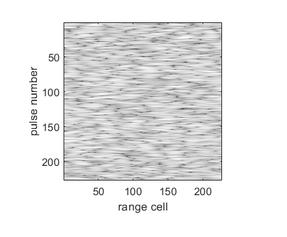
The heatmap below is a target at 10.4 dB SNR and is located at (x=171, y=196)

enter image description here

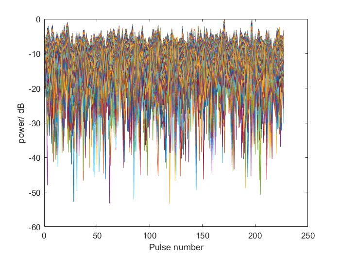
And the corresponding plot of the same RDM is here: enter image description here

$\endgroup$
11
  • $\begingroup$ In order to help we're going to need more information. Plots and some code will allow a deeper look into what you may be doing wrong. You should definitely be seeing a 10 dB target at the front of the antenna at your final detection stage. $\endgroup$
    – Envidia
    Commented Jan 23, 2023 at 20:27
  • $\begingroup$ hi @Envidia, I have included my code and example plots, thanks for your help :) $\endgroup$
    – spacey
    Commented Jan 23, 2023 at 21:25
  • $\begingroup$ Could you also please post an example of a "correct" result? I also noticed that you have a random range setting. Do not do this while trying to confirm your desired behavior. $\endgroup$
    – Envidia
    Commented Jan 24, 2023 at 4:50
  • $\begingroup$ hi, @Envidia, I'll get rid of the random range and velocity. The example I posted was what I expect a 10 dB target to look like, but I've been told it needs to be more visible or 'brighter' than that. For that to happen, I would need the noise spikes to not be so comparable to the target peak but am unsure if that is the problem. $\endgroup$
    – spacey
    Commented Jan 27, 2023 at 14:14
  • $\begingroup$ I've made some modifications to your code and will post an answer soon. I don't have access to the "awgn" function at the moment so I attempted to calculate the required noise to achieve the SNR. With the code your provided, are you saying that the -45.5 dB target achieves a final SNR of 10 dB after matched filtering and the Doppler DFT? $\endgroup$
    – Envidia
    Commented Jan 30, 2023 at 3:40

3 Answers 3

1
$\begingroup$

I'm not sure you're going to get good detection performance for your example at only 10 dB signal-to-noise ratio (SNR). Detection, in general, is a tradeoff between achieving a high probability of detection on the desired signal and a low probability of false alarm on noise (erroneously declaring a noise sample as a signal detection.)

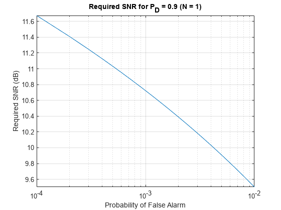
Conveniently, Mathworks has an example plot that corresponds to your case.

Required SNR for P_D = 0.9 (N = 1)

This is a plot of the required SNR to achieve a 90% probability of detection (PD) on a signal as a function of the probability of falsely declaring a signal on a noise sample. The N = 1 denotes that this is for a case without non-coherent integration.

Looking at the plot, for 10 dB SNR this would require a probability of false alarm (PFA) of approximately 4x10⁻³. Meaning that to achieve the desired detection performance you would've to accept also stating the 4 out of 1000 noise samples are also just as likely to be the desired signal. In the script provided there are many thousands of detection cell that would need to be considered (4096 x 227 = 929,792), so I would expect having to live with approximately 929,792 x 4x10-3 = 3719 false alarms.

$\endgroup$
3
  • $\begingroup$ Chirp signals enjoy strong autocorrelation. Even for lower SNR than 10dB in reception it should work reasonably well, when only AWG noise taken into account. $\endgroup$ Commented Jan 28, 2023 at 15:06
  • 1
    $\begingroup$ Only if you define SNR prior to matched filtering. If SNR is post matched filtering the modulation doesn’t matter. $\endgroup$ Commented Jan 28, 2023 at 16:08
  • $\begingroup$ @JohnBofarull What GrapefruitIsAwesome just said is one of THE fundamental results of the matched filter. There are so many resources online that tout specifics signals, such as CW, to benefit from some kind of magical correlation benefit. At the end of the day, at least for most practical radar applications, it all goes through a matched filter and the SNR is dependent on the energy put into the pulse only, which is independent of modulation. $\endgroup$
    – Envidia
    Commented Jan 30, 2023 at 5:16
1
$\begingroup$

There's a few problems with your code but you're essentially there. I haven't had the chance to do a deep-dive into your code, but I few changes gets you where you want to be.

First, you're definitely not sampling fast enough. However, given 100 MHz bandwidth of the pulse and the 10 GHz carrier, a 1 GHz sample rate still achieves bandpass filtering (a separate technique) and puts your signal in an appropriate place to match filter. If you did this knowingly then that's great, otherwise you got lucky.

Second, you're not doing the DFT-based autocorrelation correctly. In order to get the identical result of a normal convolution, you have to pad the signals to the length of the full convolution, then take the inverse DFT. I recommend that you re-write the code to use regular autocorrelations before you try to get fancy with the DFT method.

Third, be careful how you apply windowing. In this code the transmit signal is being windowed and then you window again on receive. In most radar applications, your transmit your ideal waveform then window on reception to control the sidelobes. Having said that, you're also not accounting for the loss in SNR due to windowing, which can easily be in the order of 2-4 dB depending on the window. Again, avoid applying windows until you can see the expected results without them.

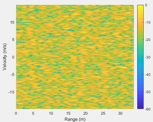
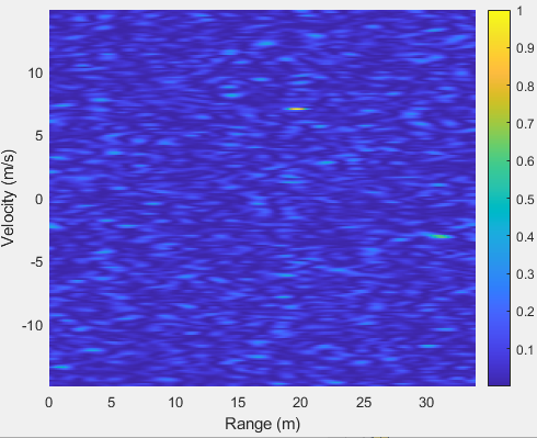
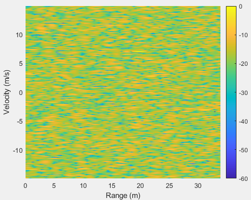
Finally, when it comes to plotting, perception can make the difference. I set the target to 20 m with a radial velocity of 7 m/s. When plotting on a dB scale you get the following using your code:

enter image description here

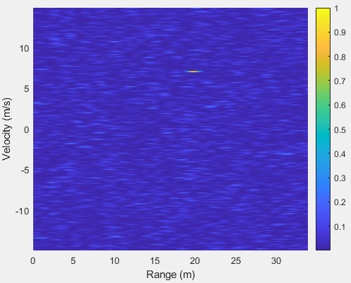
Now if you plot this in linear scale, you get

enter image description here

You can see that in linear scale, it is quite easy to distinguish the target visually.

Regarding the match filtering, I modified your code to perform the filtering using a cross-correlation and both in log-scale and linear scale you see

enter image description here enter image description here

You can see that the noise is "more flat" than the previous figures and the target is very clear. Again I haven't done the detailed analysis but it has to do with doing the DFT-based filtering incorrectly.

Finally, here's the modified code (please don't mind that I didn't bother with cleanup):

close all;
clearvars;

rng(7); % Use a static seed for repeatable results


fc=10E9;       % carrier frequency 

c=3E8;        % speed of light 

lambda=c/fc;  % wavelength

PRF=2000;     

PRI=1/PRF;    % time from pulse to pulse 


fs=1000e6;    % sampling frequency 

ts=1/fs;

t=0:ts:(PRI/122)-3*ts; % only sampling to 4096 samples

B= 100e6;                    %bandwidth 5e7

Tp=300/B;                    % setting the time bandwith product to 300

r=(c.*t)./2 ;                

k=B/Tp;                    % chirp rate 

N= 227;                    % number of pulses

T = length(t);      

Vmax=14;

v= linspace((-lambda*PRF/4),(lambda*PRF/4),N);

% V0 =Vmax*(-1+2*rand(1,1));         % target velocity
V0 = Vmax/2;

Rmin= 1;                                 % to avoid wrap around

Rmax= 33;

% R0 =Rmin + (Rmax-Rmin).*abs(rand(1,1));      % target range 
R0 = 20;
Rcell=round((2*R0/(c*ts))+1);                       % target range based on cell number

Vcell=round((N-1).*(V0+(Vmax+1))./(2*(Vmax+1))+1); % target velocity based on cell number

A0= 0;        % target acceleration


st=rectpuls((t-(Tp/2))/Tp).*exp(1i*2*pi.*(fc.*(t-Tp/2) +0.5*k*(t-Tp/2).^2)); % transmit signal for single lfm pulse 

% st(1:3000)=st(1:3000).*hanning(3000,'symmetric')';%   


z=0:N-1;

Rt= R0 - (V0.*(z)*PRI) -(A0.*(z)*PRI.^2)./2 ;     % target range at each pulse

tau=(2.*Rt./c)';

sr=(rectpuls((t-(Tp/2)-tau)./Tp).*exp(1i*2*pi.*(fc*(t-Tp/2 -tau) + 0.5.*k.*(t-Tp/2 -tau).^2))); %return signal 


% Add AWGN manually
preSNR = -45.5;
snrFactor = 10^(preSNR/10);

% Calculate average power
avgPower = mean(abs(sr.').^2);
noisePower = avgPower./snrFactor;
srr = sr + sqrt(noisePower(1)/2).*(randn(size(sr)) + 1i.*randn(size(sr)));
%     srr=awgn(sr,-45.5,'measured');

h=1:N;

srrW=fft((srr(h,:)./norm(srr(h,:))),[],2);                          % FFT of normalised return echo

stW=conj(fft(st./norm(st)));                                         %fft of normalised transmitted echo 

% for j=1:N
%         correlation(j,:)=stW.*srrW(j,:);                    %matched filtering 
% 
% end
% 
% matchedfilter=(ifft((correlation),[],2));
% 
% 
% for u=1:T
% 
% 
%        matchedfilter1(:,u)=(hanning(N,'symmetric').*matchedfilter(:,u));
% 
%        rangedoppler(:,u)= (1/N)*fftshift(fft(matchedfilter1(:,u),[],1),1);
% 
% end

%% Random internet guy's match filtering

for i = 1:N
    
    [rangedoppler(i,:), lags] = xcorr(srr(i, :), (st));
    testRDM(i,:) = rangedoppler(i, lags >= 0);
    
end

testRDM = fft(testRDM, N, 1);
rangedoppler = fftshift(testRDM, 1);

%% 
rangedoppler1=abs(rangedoppler(:,1:227)).^2;                      % cropped to 227x227 for CNN input


rangedoppler2=rangedoppler1./max(max(rangedoppler1));        % normalising


MeanNoisepower=10*log10(mean(mean((rangedoppler2(220:227)))));    % sampled at edge of map away from targets

SNR=MeanNoisepower;                                               % as target power will be 0 dB, just need noise power


%% Plot the RDM

rangeBinAxis = c/(2*fs).*(0:size(rangedoppler, 2) - 1);
velocityBinAxis = (PRF/N)*lambda/2.*(-size(rangedoppler, 1)/2:size(rangedoppler, 1)/2 - 1);

figure;
surf(rangeBinAxis(1:227), velocityBinAxis, 10*log10(rangedoppler2));
xlabel("Range (m)");
ylabel("Velocity (m/s)");
view(0, 90);
shading flat;
axis tight;
colorbar;
caxis([-60 0]);

% Show the RDM in linear scale
figure;
surf(rangeBinAxis(1:227), velocityBinAxis, rangedoppler2);
xlabel("Range (m)");
ylabel("Velocity (m/s)");
view(0, 90);
shading flat;
axis tight;
colorbar;


% imagesc((rangedoppler2))

% clim([-60 0])                                                     % have to keep the limit to -60 dB

% colormap("gray")

% truesize

figure;
plot(10*log10(rangedoppler2))
ylim([ -60 0])
$\endgroup$
8
  • $\begingroup$ thank you for your edits, @Envidia. I can see the difference in the plots very easily now. I have changed my code with your edits, including applying the tapering window to the receive signal and not the transmit one. I think I didnt name my doppler windowing correctly, but I have edited my original post now, so hopefully it clears up confusion about which dimension I applied the windows in. As a side note, for my project, I have to use windows in both dimensions and the RDMs have to be in dB also. $\endgroup$
    – spacey
    Commented Feb 1, 2023 at 17:12
  • $\begingroup$ I am also wondering if I am measuring my output SNR incorrectly, which could be why the SNR is having such drastic jumps at a supposed 10 dB output. P.S. the 55.5 dB signal processing gain is very consistent for higher SNR outputs but becomes inconsistent from around 11dB downwards :) $\endgroup$
    – spacey
    Commented Feb 1, 2023 at 17:14
  • $\begingroup$ @spacey How are you calculating that 55.5 dB processing gain? Because there's about a 7-8 dB SNR gain I've been chasing myself in your code :) $\endgroup$
    – Envidia
    Commented Feb 3, 2023 at 5:53
  • $\begingroup$ @spacey And also keep in mind that you're also keeping track of losses. Windowing introduces SNR losses, especially with 2D windows. $\endgroup$
    – Envidia
    Commented Feb 6, 2023 at 3:40
  • $\begingroup$ apologies for the late reply @Envidia ! it's 10log10(3000)(the length of the signal) + 10log10(227) (the number of pulses), which comes out at 58 dB but with the windows I have applied, it's around 55 dB. I should say that that's with the awgn function :) $\endgroup$
    – spacey
    Commented Feb 6, 2023 at 23:34
0
$\begingroup$

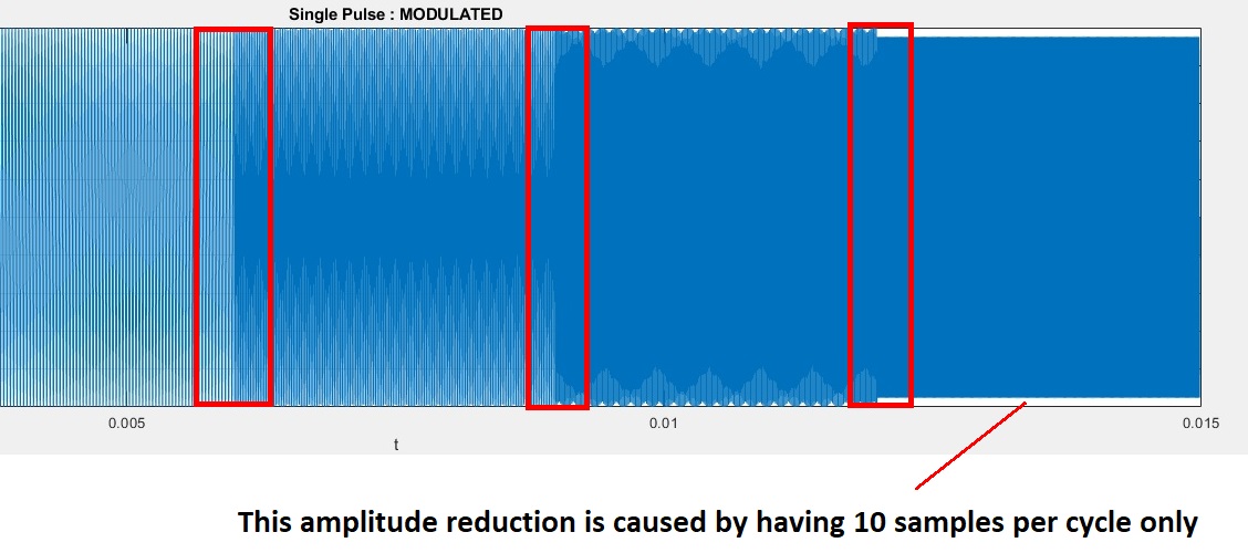
The primary point causing Just Noise is that you have fc=10e9 and fs=1e9 Heavy Undersampling.

Basically you don't have signal.

Let's build the signal :

close all;clear all;clc;

I am going to build the pulse, add noise, and you can take it from there :

1.- Start Parameters

I have divided fc and fs by 1e6 because before generating lots of samples we have to make it fly. Upsacling again is easy.

fc=1e4;         % [Hz] carrier frequency 
c=3e8;           % [m/s] speed of light 
lambda=c/fc;  % [m] wavelength

PRF=20;         % [Hz] Pulse Repetition Frequency
PRI=1/PRF;    %  [s] Pulse Repetition Interval

% fs=1e9 and fc=10e9 causes strong alias. 
% The resulting signal is meaningless with such low sampling frequency.

fs=1e2*fc;       % [Hz] sampling frequency 
dt=1/fs;          % [s] time step

D=.3                % duty cycle

t=dt*[0:dt:1];  %  ??  :(PRI/122)-3*ts; % only sampling to 4096 samples

B= 10;                    % [Hz] bandwidth 
Tp=300/B                    % setting the time bandwith product to 300

r=(c.*t)./2;            % chirp rate   
k=B/Tp                  
N= 20                   % number of pulses
T = length(t);      

Distance Velocity Acceleration Parameters

Not using the following lines :

% vmax=14;
% v= linspace((-lambda*PRF/4),(lambda*PRF/4),N);
% V0 =vmax*(-1+2*rand(1,1));         % target velocity
% Rmin= 1;Rmax= 33;                 % to avoid wrap around
% R0 =Rmin + (Rmax-Rmin).*abs(rand(1,1));      % target range 
% Rcell=round((2*R0/(c*dt))+1);                       % target range based on cell number
% Vcell=round((N-1).*(V0+(vmax+1))./(2*(vmax+1))+1); % target velocity based on cell number
% a0= 0;        % target acceleration

%    ...

% grid on;xlabel('t');ylabel('st');title('st : transmitted signal on antenna')

% st1=st(1:3000).*hanning(3000,'symmetric')';
% z=0:N-1;

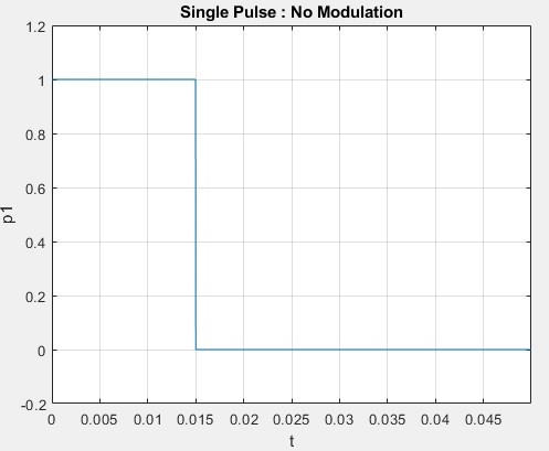
2.- Single Pulse, no modulation, no chirp

p1=[ones(1,floor(D*PRI/dt)) zeros(1,floor((1-D)*PRI/dt))];
t1=[0:dt:PRI-dt];
figure;
plot(t1,p1); grid on; xlabel('t');ylabel('p1');title('Single Pulse : No Modulation')

001

T1 is not

T1=t1(end) % = .04999  % [s] single pulse cycle 

T1 is t_stop - t_start there's a tiny dt related difference that upon several cycles derails the pulse signal.

T1=sum(numel(t1)*dt)

3.- Fix for the amount of pulses

Since you have decided the amount of pulses needed (I set it to 20, to simplify) change it accordingly, in your initial script t(end)=0.04096. If you need N pulses then t has to last at least N*T1*PRI = 1 second.

T1d=t1(floor(D*numel(t1)))+dt   % [s] pulse duty cycle 

4.- Pulse Modulation

f1=fc;f2=B*fc;

It's good practice to generate frequency-changing pulses with adjacent samples avoiding abrupt trips.

One way to do this is to step the chirp frequency

fm=linspace(f1,f2,5)  % [Hz]

Tm=1./fm                 % [s]

How many samples available per duty cycle

nTd1=round(T1d/dt)

How many samples available per frequency step

nt1=round(T1d/dt)/numel(fm)

If just 1 cycle per frequency step, it would be these amount of samples per frequency step

Nsamples_per_cycle=floor(Tm/dt)

How many cycles per frequency step

nt2=floor(nt1./Nsamples_per_cycle)

Round down to have smooth transitions between frequency steps. This can be improved to make 1st derivative to also have smooth transitions.

How many cycles per frequency step

nt2=floor(nt1/sum(floor(Tm/dt)))

Assigning same amount of samples, kind of, to each frequency step

floor(Nsamples_per_cycle.*nt2)

The following for loop prevents the amplitude of adjacent step frequencies having sharp changes.

next_shift_sign=1;
st0=[];

for s1=1:1:numel(fm)
    s_step=next_shift_sign*sin(2*pi*fm(s1)*[0:1:(nt2(s1)*Nsamples_per_cycle(s1))]*dt);
    
    diff_step_end=s_step(end)-s_step(end-1);
    last_sample=s_step(end);
    
    d2t_case=0;
    if diff_step_end>0 & last_sample>=0 % climbing and last_sample>=0
        d2t_case=1;
    end
    if diff_step_end>0 & last_sample<=0  % climbing and last_sample<=-sin(2*pi*fm(1)*dt)
        d2t_case=2;
    end
    if diff_step_end<0 & last_sample>=0   % falling and last_sample>=sin(2*pi*fm(1)*dt)
        d2t_case=3;
    end
    if diff_step_end<0 & last_sample>=0   % falling and last_sample<=0 
        d2t_case=4;
    end
       
    switch d2t_case
        case 1
            k2=1;
            while s_tep(end-k2)>-sin((2*pi*fm(1)*dt))  % climbing and last_sample>=0 : too many samples
                k2=k2+1;
            end
            s_step(end:-1:end-k2)=[];
            
        case 2
            b1=[];
            k2=1;
            while  sin(2*pi*fm(s1)*nt2(s1)*(Nsamples_per_cycle(s1)+k2)*dt)<-sin((2*pi*fm(1)*dt))  % climbing and last_sample<=0 : not enough samples
                k2=k2+1;
                b1=[b1 sin(2*pi*fm(s1)*nt2(s1)*(Nsamples_per_cycle(s1)+k2)*dt)];
            end
            s_tep=[s_step b1];
            
        case 3
            b1=[];
            k2=1;
            while sin(2*pi*fm(s1)*nt2(s1)*(Nsamples_per_cycle(s1)+k2)*dt)<-sin((2*pi*fm(1)*dt))  % falling and last_sample>0 : not enough samples 
               k2=k2+1;
               b1=[b1 sin(2*pi*fm(s1)*nt2(s1)*(Nsamples_per_cycle(s1)+k2)*dt)];
            end
            s_tep=[s_step b1];
            
        case 4
            k2=1;
           while abs(s_tep(end-k2))>sin((2*pi*fm(1)*dt))  % falling and last_sample<=0 : too many samples
                k2=k2+1;
           end
           s_step(end:-1:end-k2)=[];
            
        otherwise
            
    end
    
    if (s_step(end)-s_step(end-1))<0
        next_shift_sign=-1;
    else
        next_shift_sign=1;
    end
    
    st0=[st0 s_step];
    
end

t2=dt*[0:numel(st0)-1];
figure;
plot(t2,st0);
grid on; xlabel('t');ylabel('st0');title('Single Pulse : MODULATED, No Targets')

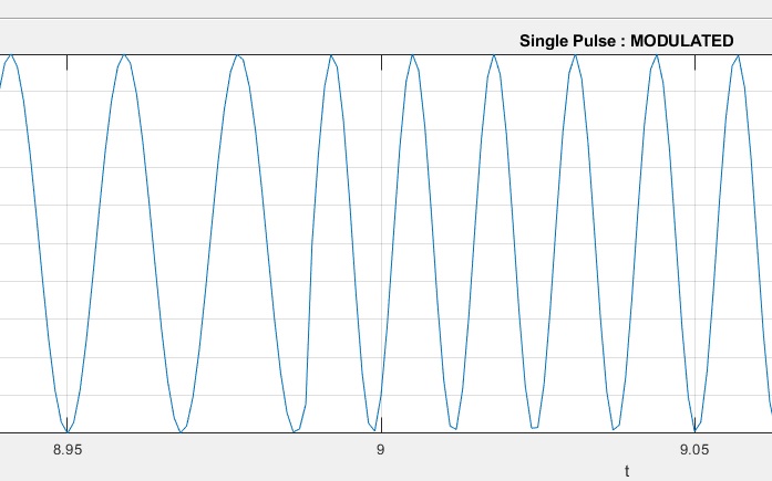
enter image description here

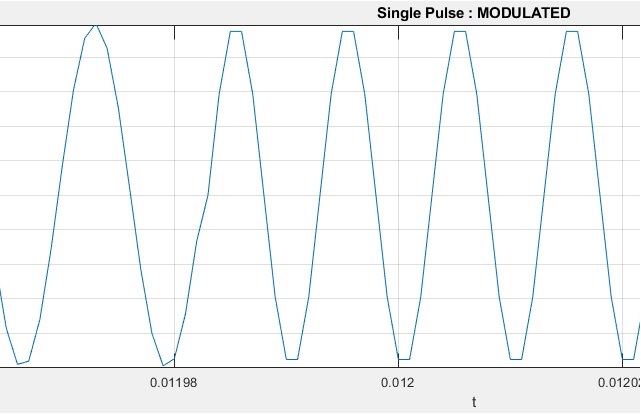
enter image description here

enter image description here

Another way that I am not getting into in this answer, would be keeping constant the amount of cycles per frequency step.

5.- Assembling Duty Cycle and Guard Interval

To discern target locations, for each pulse, whatever is received after the Duty Cycle has to be ignored.

This is the time reference for the Guard Interval

t3=[t2(end):dt:PRI-dt];

time reference for a complete pulse

tp1=[t2 t3];

p1=[st0 zeros(1,numel(t3))];

6.- Transmitted power

Ptx=mean(st0.*conj(st0))  % ~.5W transmission

figure;
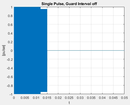
plot(tp1,p1);
grid on;xlabel('t');ylabel('|pulse|');title('Single Pulse, Guard Interval off')

004

enter image description here

I am not going to implement doppler shift caused by the random velocities that you generate in the question.

If interested please let me know, or ask another question, and I will answer accordingly.

Here you could concatenate multiple pulses

However a radar design has to start with discerning what max range is not going to cause false alarms.

Delayed signals beyond one pulse should be weak enough to neglect them. This also meaning, whatever happens in one pulse cycle should not spill over to time adjacent pulses.

7.- Received Signal : Let's assume for instance 30dB down

L_channel=-20   % [dB]

sr=10^(L_channel/10)*p1;

Because I have switched off the pulse throughout the guard interval and no targets yet, for the following calculation there's no need to include the zero samples.

Just keep the transmitter on in the Guard Interval, then when no targets, one can use the entire pulse, not just the duty cycle, for 'dry' (no targets) calculations.

8.- Adding noise

45dB is a good SNR so it's probably on transmitting antenna.

Changing 45dB to 10dB more realistic, MEASURE SNR ON RECEPTION

sr received pulse

With Communications Toolbox

% sr=awgn(sr,-45.5,'measured'); 

Without Communications Toolbox

Psr=10^(L_channel/10)*mean(st0.*conj(st0))  
SNR=10   % [dB] RECEPTION

Pn=Psr/10^(SNR/10)  % signal power
n_var=Pn               % AWGN noise standard deviation is noise power (Z0=1)
n=rand(1,numel(sr));n=n-mean(n);
% n_std=n_var^.5

a1=(Pn2/Pn)^.5
n=1/a1*n;

check, it should be the expected 10dB on reception

Psr/mean(n.*conj(n))

sr2=sr+n;

figure;
plot(t2(1:min(numel(t2),numel(sr2))),sr2(1:min(numel(t2),numel(sr2))));
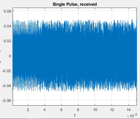
grid on;xlabel('t');ylabel('|pulse|');title('Single Pulse, received')
axis([0 t2(end) -1.2 1.2])

enter image description here

9.- If you do not add further comment I am going to stop here and you can link from this point on with your code, starting with the following lines.

h=1:N;
srrW=fft((srr(h,:)./norm(srr(h,:))),[],2);        % FFT of normalised return echo
stW=conj(fft(st./norm(st)));                           %fft of normalised transmitted echo 
...

10.-

Now there's

  • NO ALIAS
  • a concise time reference
  • a working pulse
  • Clear difference between duty cycle and the guard interval

Now you can add targets as well as pick up echos, and you can change the SNR on Reception.

NOW take the entire cycle : Duty Cycle and Guard Interval to calculate SNR and detect because target reflections should arrive within the Guard Interval of same pulse that has caused them.

$\endgroup$

Your Answer

By clicking “Post Your Answer”, you agree to our terms of service and acknowledge you have read our privacy policy.

Not the answer you're looking for? Browse other questions tagged or ask your own question.